Julia tutorial during Social Simulation Conference 2022
Introduction
During SSC2022 Conference together with Rajith Vidanaarachchi and Przemysław Szufel I am going to give An introduction to agent-based simulations in the Julia language tutorial.
During the tutorial tutorial agent-based models implemented in Julia will be discussed. Today I thought to post an example of a simple agent-based model (not covered during SSC2022) that shows one of the challenges of designing agent-based models.
The post was written under Julia 1.8.0, DataFrames.jl 1.3.5, and Plots.jl 1.32.0.
The problem
I want to create a simulation of genetic drift in Julia.
The idea of the model is as follows. On a rectangular grid we initially randomly
put agents of two types (I will use true and false to denote them). In one
step we pick a random agent and change its type to the type of one of its
neighbors. We will want to check, using simulation, if in the long run all
agents end up having the same color and how long it takes, on the average,
to reach this state.
A crucial design decision when modeling this problem is how we define neighbors
of an agent. Some classical definitions are Moore or von Neumann
neighborhoods on a torus. However, in the experiment today I assume
that if I have an agent in location (x,y) it has four neighbors on diagonals:
(x+1, y+1), (x-1, y+1), (x+1, y-1), (x-1, y-1) (we assume the simulation
is run on a torus, so left and right edge, and top and bottom edges of the grid
are glued together). I want to see what consequence this definition of the
neighborhood has on the results of the simulation.
An initial test
Let us start with an implementation on a grid of size 10 times 10 and plot the dynamics of the system. Here is the code running 30,000 steps of the simulation and want to see if we end up with all cells having the same type:
using Random
using Plots
Random.seed!(1234)
m = rand(Bool, 10, 10)
anim = @animate for tick in 1:30000
    x, y = rand(axes(m, 1)), rand(axes(m, 2))
    nx = mod1(x + rand((1, -1)), size(m, 1))
    ny = mod1(y + rand((1, -1)), size(m, 2))
    m[x, y] = m[nx, ny]
    heatmap(m, legend=false, size=(400, 400), title=tick)
end every 100
gif(anim, "anim_fps15.gif", fps=15)
The code saves the result as an animated GIF file that you can see below:
Surprisingly, we reach a steady state that consists of 50% of true and 50%
of false cells. This teaches us that one should be careful when designing
ABM models, as small changes in the code can lead to significant changes it
the behavior of the model. The point is that our neighborhood consisting of
four diagonal neighbors defines two disjoint sets of cells on a square having even
size. In von Neumann neighborhood, which also consists of four negihbors
(but top-down and left-right) we would not have such a problem.
Let us investigate our flawed model for different sizes of the grid.
Checking different sizes of a grid
We want to check how often different steady states are reached for different sizes of the grid and how long it takes to reach these steady states.
Before we can do it we first need to think of some rule that detects that the simulation has reached a steady state and at the same time is cheap to check.
There are many ways to do it. Let me propose the following reasoning here. If we
have a square toroidal grid whose side is d we have 2d^2 pairs of nodes that
are neighbors. To see this note that we have d^2 agents and each node has 4
neighbors; in other words the grid is a 4-regular graph on d^2 nodes, so it
has 2d^2 edges.
Notice that if we in a continuous sequence visit every edge of this graph at
least once and we always see the same color on both ends of the edge we have
reached a steady state. Additionally, each edge of the graph is visited with
the same probability in each tick. Now assume that we run this process for t
ticks. The probability that we have never picked some concrete edge during this
time at is (1-1/(2d^2))^t. Since we have 2d^2 such edges, by union bound,
the probability that we have not picked at least one of the edges is less than
2d^2(1-1/(2d^2))^t. We want t to be large enough so that this probability is
small. Assume that we want this probability to be less than 1e-6. We thus
need to find a minimum t that satisfies 2d^2(1-1/(2d^2))^t<1e-6 as a
function of d. Using the approximation log(1+x) ≈ x for x close to 0 we
get that t > 2d^2*log(500_000d^2). For example for d=10 we can compute that
t must be at least 3546. In other words if for 3546 steps we do not make
any swaps of agent’s state we are very likely to have reached a steady state.
Using this derivation let us put our simulation in a function:
function runsim(d)
    m = rand(Bool, d, d)
    tick = 0
    lastchange = 0
    t = 2d^2*log(500_000d^2)
    while lastchange < t
        tick += 1
        x, y = rand(axes(m, 1)), rand(axes(m, 2))
        nx = mod1(x + rand((1, -1)), size(m, 1))
        ny = mod1(y + rand((1, -1)), size(m, 2))
        old = m[x, y]
        new = m[nx, ny]
        if old == new
            lastchange += 1
        else
            lastchange = 0
        end
        m[x, y] = new
    end
    class=sum(m)
    if iseven(d)
        @assert allequal(m[i, j] for i in 1:d, j in 1:d if iseven(i+j))
        @assert allequal(m[i, j] for i in 1:d, j in 1:d if isodd(i+j))
    else
        @assert allequal(m)
    end
    return (;d, tick, class)
end
Notice, that I have additionally added @assert checks that make sure
that indeed we have reached a steady state. However, we make this check only
once as it is expensive.
In the output the class value is number of true cells in the grid.
Let us now run this simulation for d ranging from 4 to 11 and 2048 times
for each size of the grid and keep the results in a data frame:
julia> using DataFrames

julia> using Statistics

julia> df = DataFrame([runsim(d) for d in 4:11 for _ in 1:2048])
16384×3 DataFrame
   Row │ d      tick   class
       │ Int64  Int64  Int64
───────┼─────────────────────
     1 │     4    595      8
     2 │     4    556      8
     3 │     4    570      8
   ⋮   │   ⋮      ⋮      ⋮
 16382 │    11  16112      0
 16383 │    11  17230    121
 16384 │    11  20914      0
           16378 rows omitted
First, we want to analyze if indeed for even grid size we have three different possible outcomes and for odd sized grid we have two possible steady states:
julia> combine(groupby(df, [:d, :class], sort=true), nrow, :tick .=> [mean, std])
20×5 DataFrame
 Row │ d      class  nrow   tick_mean  tick_std
     │ Int64  Int64  Int64  Float64    Float64
─────┼────────────────────────────────────────────
   1 │     4      0    504    604.919     68.1656
   2 │     4      8   1017    605.345     65.5917
   3 │     4     16    527    607.355     69.8784
   4 │     5      0   1015   1309.11     388.342
   5 │     5     25   1033   1341.45     415.868
   6 │     6      0    528   1853.26     425.983
   7 │     6     18   1038   1844.34     409.991
   8 │     6     36    482   1879.57     458.587
   9 │     7      0   1002   4077.81    2059.13
  10 │     7     49   1046   3901.26    1777.57
  11 │     8      0    521   4739.05    1562.39
  12 │     8     32   1027   4620.13    1481.39
  13 │     8     64    500   4717.03    1626.72
  14 │     9      0   1025   9825.73    5347.35
  15 │     9     81   1023  10069.5     5665.56
  16 │    10      0    491  10331.5     4139.39
  17 │    10     50   1075  10233.4     4008.2
  18 │    10    100    482  10469.8     4337.41
  19 │    11      0   1035  21127.0    12885.3
  20 │    11    121   1013  21374.3    13331.7
Indeed this is a case. Moreover we note that:
- for even-sized grids having a mixed steady state is as likely as having a homogenous steady state (this is expected);
- increasing grid size increases the time to reach the steady state (this is expected);
- time to reach each steady state, for a given
dhas approximately the same distribution (we have calculated mean and standard deviation of this time to confirm this; again this is expected).
Finally let us calculate the average time to reach steady state by d and plot
it:
julia> res = combine(groupby(df, :d, sort=true), :tick => mean)
8×2 DataFrame
 Row │ d      tick_mean
     │ Int64  Float64
─────┼──────────────────
   1 │     4    605.757
   2 │     5   1325.42
   3 │     6   1854.93
   4 │     7   3987.64
   5 │     8   4674.04
   6 │     9   9947.51
   7 │    10  10312.6
   8 │    11  21249.3

julia> scatter(res.d, res.tick_mean, legend=nothing, xlab="d", ylab="mean ticks")
The resulting plot is:
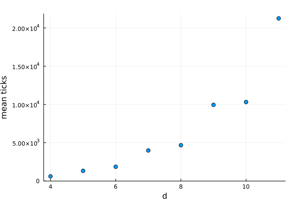
What is interesting is that there is much bigger increase of the time when we
move from even to odd d than when moving from odd to even d. What is the
reason for this? The reason is that for odd d the agents’ graph is connected.
There is a single component having d^2 elements. While for even d we have
two connected components, each having d^2/2 size. We have just learned that it
is much faster to independently reach a steady state for component of size
d^2/2 twice than to reach a steady state of a single component of size d^2.
Conclusions
I hope you enjoyed the post both from ABM and Julia language perspectives. I tried to avoid going into too much detail, both from mathematical and implementation side of the model. If you have any questions please contact me on Julia Slack or Julia Discourse.