A basic SIR model using agent-based approach in Julia
Introduction
Recently I have written a blog post about a simple agent-based model in finance domain. This is a follow up post in preparation for Social Simulation Week 2020 workshop on agent-based modeling using the Julia language that will be given by Przemysław Szufel and me.
This time I have decided to present a simple SIR model implementation using an agent-based design.
The Julia codes presented in this post are also available as a Jupyter notebook here.
The SIR epidemic model specification
We assume that we have a finite population of n agents that live on a discrete
torus that has (xdim, ydim) size.
If you have not heard of such a model of the space then imagine it is a (xdim,
ydim) chessboard whose top and bottom, as well as left and right borders are
glued together. Thus you never fall-off the board — you can travel e.g. to the
right infinitely as the space is wrapped. Here is a plot illustrating the
gluing process:

and here is the end result 😄:

The torus model of the space is quite popular in simple agent-based models as it is similar to a square grid, but does not have borders nor corners.
We assume that agents independently move around our torus in a discrete time.
Some agent in time moment tick randomly chooses to move up/stay/down and
left/stay/right (so in total there are nine possibilities, one of which is to
stay in place).
In particular the above rules mean that at some moment in time several agents can occupy the same cell. This is where the SIR epidemiological model comes into play. We assume that there is some disease and an agent can be in one of four states:
- susceptible: S
- infected: I
- recovered: R
- dead
There are the following rules for moving between states in our model:
- if in some tick a susceptible agent is on the same cell in the grid as an infected agent then the susceptible agent becomes infected;
- infected agent stays infected for
durationperiods after which time the agents becomes dead with probabilitypdeathand otherwise becomes recovered; - recovered and dead agents do not change their state except that recovered agents are still allowed to move on the grid.
Initially we assume that infected number of agents is in an infected state.
We run the simulation as long as there is at least one infected agent.
In this post I present an implementation of an agent-based simulation that captures the dynamics of this system and allows us to track changes of its state in time.
Implementation of the model
This post is written under Julia v1.5.0, PyPlot v2.9.0, and StatsBase v0.32.2 (normally I recommend to make sure that you have exactly the given versions of the packages installed, but in this case I only use their basic functionality so you can safely assume that any version should work). I assume that you use just Julia REPL (in a terminal or in an IDE like VS Code), but all examples should also work in Jupyter notebook.
To import the required packages write:
using StatsBase
using PyPlot
If you get an error loading the packages most likely they are not installed. In this case add them by running:
using Pkg
Pkg.add("StatsBase")
Pkg.add("PyPlot")
Let us now move to definitions of data types that we will use in our model:
@enum AgentType agentS agentI agentR agentD

struct Agent
    x::Int # location of an agent in x-dimension
    y::Int # location of an agent in y-dimension
    type::AgentType # type of an agent
    tick::Int # moment in time when agent entered type `type`
end

mutable struct Environment
    grid::Matrix{Vector{Int}} # for each cell of a grid a vector of numbers
                              # of agents currently occupying a given cell
    agents::Vector{Agent}     # a vector of all agents
    duration::Int             # metadata: how long agent stays in infected state
    pdeath::Float64           # metadata: probability of death of an agent after
                              # being infected
    stats::Dict{AgentType, Vector{Int}} # a dictionary storing number of agents
                                        # of each type in consecutive ticks
                                        # of the simulation
    tick::Int                 # counter of the current tick of the simulation
end
We have created three types:
AgentTypewhich is just an enumeration allowing us to refer to the type of the agent (agentSfor susceptible,agentIfor infected,agentRfor recovered, andagentDfor dead); thus later in the code we can writeagentS,agentIetc. specify the type of an agent;Agentis a structure holding information about a single agent; note that we create this type usingstructkeyword, which means that it is immutable (it will have an impact how we should work with such a structure as will be seen later in the code);Environmentis a mutable structure holding global information about the simulation state; this time we make this structure mutable, which means that we can change the values of variables stored in it.
Let us now move to a function that initializes the state of the simulation:
function init(n::Int, infected::Int,
              duration::Int, pdeath::Float64, xdim::Int, ydim::Int)
    grid = [Int[] for _ in 1:xdim, _ in 1:ydim]
    agents = [Agent(rand(1:xdim), rand(1:ydim),
                    i <= infected ? agentI : agentS, 0) for i in 1:n]
    for (i, a) in enumerate(agents)
        push!(grid[a.x, a.y], i)
    end
    stats = Dict(agentS => [n - infected],
                 agentI => [infected],
                 agentR => [0],
                 agentD => [0])
    return Environment(grid, agents, duration, pdeath, stats, 0)
end
We see that essentially it populates the Environment container. Note
that initially there are infected number of agents in the agentI state,
and the rest of them is in agentS state. Each agent initially gets a random
location on the grid. We also make sure to correctly initialize the grid and
stats variables.
As we have noted above the Agent container is immutable. Therefore we have to
define functions that take an Agent object and return a new Agent object
if the Agent is to change its state.
die(a::Agent, tick::Int) = Agent(a.x, a.y, agentD, tick)

recover(a::Agent, tick::Int) = Agent(a.x, a.y, agentR, tick)

infect(a::Agent, tick::Int) = Agent(a.x, a.y, agentI, tick)

move(a::Agent, dims::Tuple{Int, Int}) =
    if a.type == agentD
        a
    else
        Agent(mod1(a.x + rand(-1:1), dims[1]),
              mod1(a.y + rand(-1:1), dims[2]),
              a.type, a.tick)
    end
As we have described above an agent can change its type, which is handled by
the die, recover, and infect functions, and it can move, which is handled
by the move function. Let us note a few things about the implementation of
these functions:
- we use a short-form definitions of these functions of the form
f(x) = expr; this is useful when a function body is just a single expression (in particular note that theif-elseclause is a single expression — as shown in themovefunction); - in the
movefunction thedimsargument are the dimensions of the grid and the expressionsmod1(a.x + rand(-1:1), dims[1])andmod1(a.y + rand(-1:1), dims[2])handle the movement of the agent to one of the nine new positions above and themod1functions makes sure that if we move out of the boundary of the grid the movement is properly wrapped (e.g.mod1(0, 10)is10andmod1(11, 10)is1);
In each tick of the simulation we first update the type of the agents, which is handled by the following function:
function update_type!(env::Environment)
    tick = env.tick
    for (i, a) in enumerate(env.agents)
        if a.type == agentI
            if tick - a.tick > env.duration
                env.agents[i] = if rand() < env.pdeath
                    die(a, tick)
                else
                    recover(a, tick)
                end
            else
                a.tick == tick && continue
                for j in env.grid[a.x, a.y]
                    a2 = env.agents[j]
                    if a2.type == agentS
                        env.agents[j] = infect(a2, tick)
                    end
                end
            end
        end
    end
end
Note that this function’s name ends with ! which is a convention that the
function changes its env argument. In this case it changes the agent types
stored in agents field of env mutable struct.
The whole logic of the update_type! function revolves around agents that have
agentI type as they either can infect agents that have agentS type or can
either recover and become agentR or die and become agentD type.
Note that each time an agent type is changed we have to update the collection
env.agents with a new value as Agent type is immutable.
Also the condition a.tick == tick && continue might raise some questions.
We use it to make sure that agents that became sick in a given tick to not
recursively infect other agents in the same tick (in our model it has only
performance implications as we assume that agents can get infected only
if an already infected agent stays in the same cell; but this would start
to matter if we allowed e.g. a wider infection radius — which is an easy
extension to version of the model we present — as then a chain reaction
could be triggered in a single tick, and we want to avoid this).
The other collective action of agents is their movement that is defined here:
function move_all!(grid::Matrix{Vector{Int}}, agents::Vector{Agent})
    foreach(empty!, grid)
    for (i, agent) in enumerate(agents)
        a = move(agent, size(grid))
        agents[i] = a
        push!(grid[a.x, a.y], i)
    end
end
Here a notable thing is that we clear entries of a grid cache with the empty!
function for each cell of grid matrix and then populate it anew with updated
locations of the agents.
The last thing we need to do in each step of the simulation is collection of the statistics. This is a relatively simple operation and is implemented using the following code:
function get_statistics!(env::Environment)
    status = countmap([a.type for a in env.agents])
    for (k, v) in env.stats
        push!(v, get(status, k, 0))
    end
end
In this function we use the countmap function form the StatsBase.jl package to
get numbers of agents of each type in a given tick, next we use a get function
to populate env.stats dictionary. The use of get is needed as in general the
status dictionary returned by countmap does not have to contain all types of
agents (e.g. in tick one of the model agents are of type agentR or
agentD are not present).
We are now ready to define the main loop of the simulation:
function run!(env::Environment)
    while env.stats[agentI][end] > 0
        env.tick += 1
        update_type!(env)
        move_all!(env.grid, env.agents)
        get_statistics!(env)
    end
end
Note that in this function we take advantage of the fact that env is mutable
and increment tick by 1 in each step. Next we repeatedly update agents’ types,
move them and collect statistics as long as there is at least one infected agent.
Running the model
Let us try running the model for some sample parameterization. We assume to have
2000 agents living on a 100x100 grid. The duration of infection is 21 ticks,
we initially place 10 infected agents (so it is 0.2% of the total population)
and assume that 5% of agents that get infected eventually die:
e = init(2000, 10, 21, 0.05, 100, 100)
run!(e)
foreach(plot, values(e.stats))
legend(string.(keys(e.stats)))
You should get a plot similar to this one:
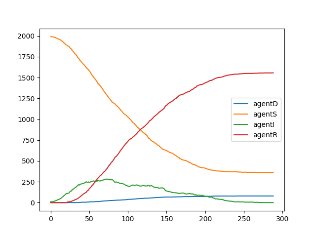
We see that the epidemics died out at around 300 ticks and around 80% of the
population went through the disease (agents that have agentS type at the end
of the simulation were unaffected).
As a second experiment let us check how does the fraction of infected agents depend on the length of the infection. Here is the code (it should run under 30 seconds):
function fraction_infected(l)
    e = init(2000, 10, l, 0.05, 100, 100)
    run!(e)
    return 1 - e.stats[agentS][end] / 2000
end

len = 5:30
runs = 16
inf = [sum(fraction_infected(l) for r in 1:runs) / runs for l in len]
plot(len, inf)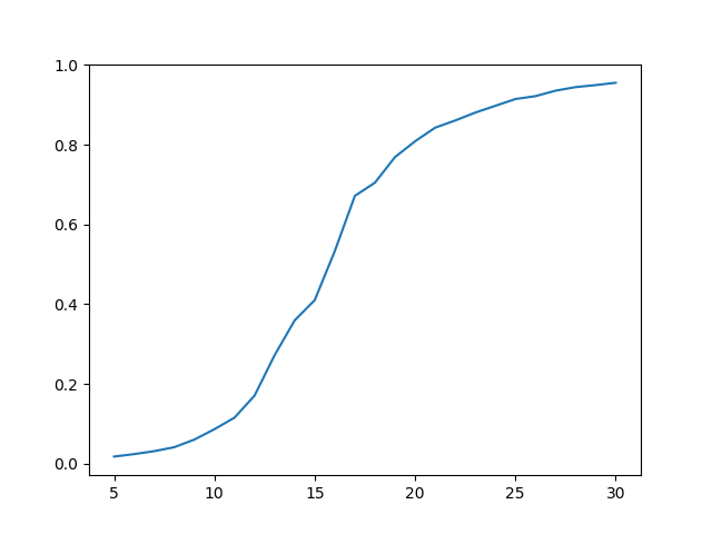
We have run the simulation for the disease length ranging from 5 to 30 with step equal to 1 and averaged out 16 runs of the simulation for each parameter (416 runs of the simulation in total). We observe that the relationship is S-shaped and the highest impact of the disease length change on number of infected agents is around fifteen ticks.
Of course these are just two samples of the analysis that can be made with this model. Feel free to change the assumptions of the model or the experiment setup if you would like to investigate it more.
Concluding remarks
In this post I have shown how you can create a simple agent-based model without having to use specialized packages. Still it is worth to know that there is e.g. an excellent Agents.jl package that provides a lot of utility data structures and functions for building agent-based simulations.
To recap the things related to the Julia language usage for building agent-based simulations I wanted to show in this post:
- you can use either
structormutable structtypes depending on what style of data management pattern you prefer (I have shown both in this post); in general the choice will have performance implications — using immutablestructwill tend to be faster in most cases — but as the Julia language is fast in general I recommend not to go for premature optimizations here, but rather use the patterns that are convenient for you as a developer; - usually it is most convenient if you create just one type of agent (here
Agent) and if you have subtypes of agents having different behavior to store this trait as a field in the this type (in our caseAgentTypeenum served as this trait); in a blog post I have written some time ago I discuss different possible patterns that could be used instead (with their performance implications), but what I show in this post should serve you well in 99% of cases from my experience; - finally let me comment that I could have easily made this simulation faster if I wanted to sacrifice code clarity (a pet pastime of many hard-core Julia uses 😄). This is a beauty of Julia that you can go really low-level in the performance critical code to optimize things (see e.g. my recent answer to this question on Stack Overflow ); however, as noted above — I usually recommend to go for such optimizations only if needed, as Julia is typically fast enough if you write the code just that follows how you think about the problem you solve, barring you do not respect general performance recommendations described here in the Julia manual.
Reader feedback
After the post I have received feedback from CGMossa with a Rust implementation of my code. I really recommend to check it out as there is a lot to learn about Rust from this code. You can find it here.