First steps with agent based modeling in the Julia language

Introduction

Recently I observe a constant raise of interest in the Julia language in community working with agent based models. I think that the reason is relatively simple (here I am probably biased, but I am really convinced about it, having used a vast number of programming languages to create such models in the past): Julia code is clean and expressive while at the same time it allows you to achieve relatively easily a decent performance.

I also think that the beauty of Julia is that you can relatively effortlessly create complex simulation models without having to use specialized packages. Most of the useful functionality is available out of the box in Julia Base. This does not mean of course, that there is a lack of specialized packages that can help you develop such models, as there is e.g. an excellent Agents.jl. I just want to say that you can go really far without much effort just by learning the core language.

In this post I want to present an implementation of a very simple model of volatility clustering on financial markets that was proposed by Rama Cont. I will discuss this model during the planned workshop on agent based modeling using the Julia language that will take place on-line during the Social Simulation Week 2020 (I will probably post more details on it when the exact schedule is out).

Additionally in the second part of the post I show an example how you can perform simple data modeling tasks using Julia.

In the examples here I use Julia 1.5, StatsBase v0.33.0, DataFrames v0.21.4, GLM v1.3.9, Optim v0.22.0, ForwardDiff v0.10.12, and PyPlot v0.2.9.0 (if you do not have much experience in setting up project environments in the Julia language have a look at this post and posts linked there). In the example of R code it was run under R 4.0.2 and e1071 version 1.7-3.

The Julia codes presented in this post are also available as a Jupyter notebook here.

The model

Our agent based model is defined as follows.

Assume we have \(n\) agents that are trading a single asset. The transactions take place in discrete time. Each agent has its individual trading threshold \(\theta_i(t)\) that evolves in time; initially \(\theta_i(1) = 0\). In each period news from the company is provided, denote it \(\varepsilon_t\). We assume that \(\varepsilon_t\) are IID following standard normal distribution. An individual agent \(i\) wants to buy an asset if the news is good enough, formally \(\varepsilon_t > \theta_i(t)\). Similarly the agent wants to sell an asset if \(\varepsilon_t < -\theta_i(t)\). In other words agents that have high \(\theta_i(t)\) are not very likely to trade, while agents that have it very close to \(0\) trade in almost every period. Also note that if \(\varepsilon_t > 0\) then agent either wants to buy or does nothing, while if \(\varepsilon_t < 0\) then agent either wants to sell or does nothing (the case of \(\varepsilon_t = 0\) is degenerated and we leave it unspecified as it will not affect our model dynamics).

By \(Z_t\) denote the sum of all buy bids minus sum of all sell bids placed by agents in period \(t\). Then we define the return of the asset in that period as \(r_t = Z_t / (n \cdot\lambda)\), where \(\lambda\) is a parameter of the model, that can be interpreted as damping factor of the returns.

Now agents observe \(r_t\) and each agent with probability \(q\) sets its \(\theta_i(t)\) to be \(|r_t|\). Observe that with this mechanism if the returns \(r_t\) are large in absolute values agents become less likely to trade in the future, while if it is close to \(0\) more trades are likely to take place in next rounds.

We will want to check if the distribution of asset returns \(r_t\) produced by this model exhibits positive excess kurtosis (as would be expected in financial markets).

In our model we have three parameters \(n\) (number of agents), \(\lambda\) (scaling factor of the returns), and \(q\) (probability to change \(\theta_i(t)\) in one round). A careful reader will note that the model has one less parameter than the one described in Cont (2007). The reason for this is explained here, and it does not affect our analysis. Additionally we will need to specify the time, as the number of ticks of the simulation, during which we will track the simulation of our model.

An implementation from the past

Several years ago (before Julia was available) I used the following implementation of the described model using the R language.

library(e1071)

cont.run <- function(time=10000, n=10000, lambda=0.05, q=0.1) {
  r <- rep(0, time)
  theta <- rep(0, n)
  eps <- rnorm(time, 0)
  for (t in 1:time) {
    if (eps[t] > 0) {
      r[t] <- sum(eps[t] > theta) / (lambda * n)
    } else {
      r[t] <- -sum(-eps[t] > theta) / (lambda * n)
    }
    theta[runif(n) < q] <- abs(r[t])
  }
  return(kurtosis(r))
}

I knew, that I am using loops, so this code would not be super efficient, but still I expected it to be reasonably good, as most of the heavy-lifting (calculation of r[t] and updates of theta) is vectorized.

A benchmark of the performance of this implementation is the following:

> system.time(cont.run())
   user  system elapsed
  2.808   0.016   2.824

So in practice (what we are going to do shortly) I had to design an experiment and leave the computations running for many hours to get any results that would allow to perform the analysis. For instance testing a full factorial design with 51 levels of \(\lambda\) and 51 levels of \(q\) would already take 2 hours assuming taking one measurement per design point (which is a very small experiment).

An implementation using the Julia language

Here is a way to rewrite the implementation of the model to Julia:

using Random
using StatsBase

function cont_run(time=10000, n=10000, λ=0.05, q=0.1)
    r = zeros(time)
    θ = zeros(n)
    pchange = zeros(n)
    for t = 1:time
        ε = randn()
        if ε > 0
            r[t] =  sum(<(ε), θ) / (λ * n)
        else
            r[t] =  -sum(<(-ε), θ) / (λ * n)
        end
        θ .= ifelse.(rand!(pchange) .< q, abs(r[t]), θ)
    end
    return kurtosis(r)
end

Let us check the performance our our code:

julia> @time cont_run();
  0.091730 seconds (25 allocations: 254.797 KiB)

julia> @time cont_run();
  0.100935 seconds (6 allocations: 234.609 KiB)

We see that it is around 30 times faster than R. Also note that I have run @time twice, as the first time compilation cost is included in the timing (in this case it turned out to be negligible).

The R and Julia codes are almost identical (translating R to Julia took me literally a few minutes). The notable differences are:

• In the line sum(<(ε), θ) I apply an anonymous function <(ε) to all elements of the vector θ, which allows me to calculate the transformed sum without doing any temporary allocations (for a reference, when I write <(ε) I define an anonymous function so that comparison x < y can be written as f = <(y) and then f(x); such a construct is called partial function application).
• I preallocate pchange vector so that later I can use rand! from Random module to generate required random numbers without allocating new memory.
• In the line θ .= ifelse.(rand!(pchange) .< q, abs(r[t]), θ) I use broadcasting assignment, again avoiding allocation of new memory in each iteration.

Note that these optimizations mean that my code does only 6 memory allocations (which you can see in the second output of @time). Usually avoiding allocations means that your code will run fast, as allocations are expensive.

Analyzing the model output

Let us perform a minimal analysis of the output of our model to showcase several packages in the Julia ecosystem. Here is the code that we will run (it is a most basic experiment design for this model, as normally you would want to include like making sure we compute statistics of a stationary distribution, or collect independent measures per design point but I do not want to overly complicate things):

function run_sim(time=10000, n=10000)
    df = DataFrame()
    for λ in range(0.01, 0.05, length=51), q in range(0.01, 0.05, length=51)
        push!(df, (λ=λ, q=q, k=cont_run(time, n, λ, q)))
    end
    return df
end

I did not have to put it in a function, but it is a good practice in Julia to wrap your code like this. Note the use of push! to populate the data frame with data. We will use this pattern again later in this post.

Let us now try to run it and do some simple visualization of the results:

julia> using DataFrames

julia> using PyPlot

julia> Random.seed!(1234); # ensure reproducibility of the results

julia> @time df = run_sim();
281.787909 seconds (58.70 k allocations: 597.163 MiB, 0.01% gc time)

julia> scatter(df.λ, df.q, 10, df.k, cmap=get_cmap("RdYlBu"));

julia> colorbar();

julia> xlabel("λ");

julia> ylabel("q");

julia> title("kurtosis");

Here is the produced plot:

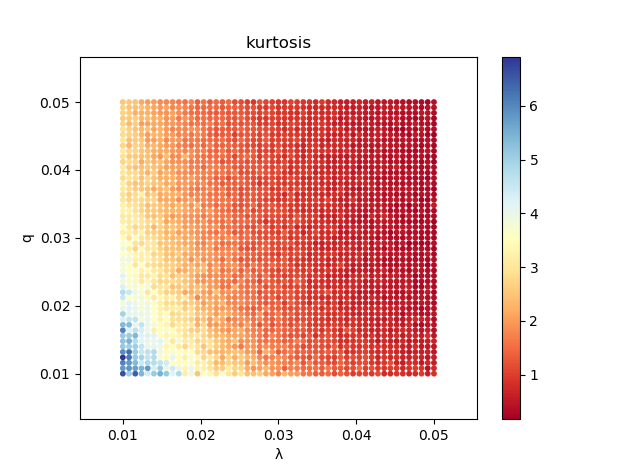
We observe that the model visually looks to be more sensitive to changes of \(\lambda\) than to changes of \(q\) and that there should be a significant interaction effect between them. In general: the more often the investors change their decision threshold and the higher the asset return damping factor is the less leptokurtic the distribution of returns is.

We can quickly check it using a metamodel of the form:

\[\text{kurtosis}\approx\alpha_0 + \alpha_1\cdot\lambda^{\alpha_2}+\alpha_3\cdot q^{\alpha_4}+\alpha_5\cdot\lambda^{\alpha_2}\cdot q^{\alpha_4}\]

Here is the code that estimates it:

julia> using GLM

julia> using Optim

julia> function best_model(df)
           function obj(x)
              f1(v) = v^x[1]
              f2(v) = v^x[2]
              return -r2(lm(@formula(k ~ f1(λ) * f2(q)), df))
          end
          return optimize(obj, rand(2) .- 0.5).minimizer
       end
best_model (generic function with 1 method)

julia> best_model(df)
2-element Array{Float64,1}:
 -0.44704271272778473
 -0.6976813327295656

julia> model = lm(@formula(k ~ (λ ^ -0.447) * (q ^ -0.698)), df)
StatsModels.TableRegressionModel{LinearModel{GLM.LmResp{Array{Float64,1}},
GLM.DensePredChol{Float64,LinearAlgebra.Cholesky{Float64,Array{Float64,2}}}},
Array{Float64,2}}

k ~ 1 + :(λ ^ -0.447) + :(q ^ -0.698) + :(λ ^ -0.447) & :(q ^ -0.698)

Coefficients:
────────────────────────────────────────────────────────────────────────────────────────────
                           Estimate  Std. Error    t value  Pr(>|t|)   Lower 95%   Upper 95%
────────────────────────────────────────────────────────────────────────────────────────────
(Intercept)              -0.333956   0.0469543    -7.11236    <1e-11  -0.426028   -0.241884
λ ^ -0.447                0.149634   0.00901133   16.6051     <1e-58   0.131964    0.167304
q ^ -0.698               -0.208741   0.00342888  -60.8773     <1e-99  -0.215464   -0.202017
λ ^ -0.447 & q ^ -0.698   0.0569654  0.00065806   86.5657     <1e-99   0.0556751   0.0582558
────────────────────────────────────────────────────────────────────────────────────────────

julia> r2(model)
0.9778978893786601

Note that in the example we find the exponents to which \(\lambda\) and \(q\) should be raised to get the best fit (which is quite good considering the resulting \(R^2\)). In particular in the line

-r2(lm(@formula(k ~ f1(λ) * f2(q)), df))

we dynamically inject the user defined f1 and f2 functions into the model formula. Similarly in

lm(@formula(k ~ (λ ^ -0.447) * (q ^ -0.698)), df)

we use exponentiation to transform the variables.

We can see that there is a significant interaction effect between the variables, as expected. As the resulting estimated function is non-linear, in order to check the range of marginal effects of \(\lambda\) and \(q\) in the domain of our design space, we will use the ForwardDiff.jl package:

julia> using ForwardDiff

julia> function get_gradients(model, df)
          prediction(x) = predict(model, DataFrame(λ=x[1], q=x[2]))[1]
          grad_df = DataFrame(λ=Float64[], q=Float64[])
          foreach(eachrow(df)) do row
              push!(grad_df, ForwardDiff.gradient(prediction, [row.λ, row.q]))
          end
          return describe(grad_df, :min, :mean, :median, :max)
       end
get_gradients (generic function with 1 method)

julia> get_gradients(model, df)
2×5 DataFrame
│ Row │ variable │ min      │ mean     │ median   │ max       │
│     │ Symbol   │ Float64  │ Float64  │ Float64  │ Float64   │
├─────┼──────────┼──────────┼──────────┼──────────┼───────────┤
│ 1   │ λ        │ -548.901 │ -90.9051 │ -62.6736 │ -20.8306  │
│ 2   │ q        │ -412.666 │ -35.1307 │ -18.6697 │ -0.973361 │

which confirms our visual observations that both variables have a negative derivative for the points in our design space and that the results are more sensitive to the changes of \(\lambda\) than of \(q\).

In terms of the performance note that the most expensive part, that was to create the df data frame, took under 5 minutes instead of estimated 2 hours in R.

Conclusion

This was a minimal showcase how you can implement a very simple agent based model using the Julia language. What I wanted to present is that the implementation of the model is as short as in e.g. R language, while at the same time you can get significant performance benefits (which is a very relevant issue when developing agent based models).

In the second part of the post I did some simple analysis of results of simulation experiment using this model to show several packages that are often used in such situations. I hope you enjoyed it!

As a final comment let me ask for some crowdsourcing :), as I want to show the participants of Social Simulation Week 2020 a comparison of several options against the Julia language. Therefore, similarly to the case of a recent post, I will be happy to update this post with codes provided by the readers to compare the complexity and performance. The challenge is to maximize speed (primary criterion) and at the same time have a relatively simple code (secondary criterion). I will benchmark and post the results of the submitted codes here. In general as we want to concentrate mostly on speed any programming language is welcome, with a restriction that we want to use CPU computing on a single thread. If you are interested please send me your implementation of cont_run function either via e-mail on Julia slack.

Appendix: Implementations provided by the readers

Here are the implementations of the model I have received from the readers.

Python

Tomasz Olczak has sent me Python ports of the code (thank you for working on it). The first naive version is almost identical to Julia code:

from numpy import zeros
from scipy.stats import kurtosis
from numpy.random import default_rng

rng = default_rng()

def cont_run(time=10000, n=10000, λ=0.05, q=0.1):
    θ = zeros(n)
    r = zeros(time)
    pchange = zeros(n)
    ε = rng.standard_normal(time)
    for t in range(time):
        if ε[t] > 0:
            r[t] = (ε[t] > θ).sum() / (λ * n)
        else:
            r[t] = -(-ε[t] > θ).sum() / (λ * n)
        θ[rng.random(out=pchange) < q] = abs(r[t])
    return(kurtosis(r))

It runs roughly 7.5 times slower than the Julia code, which you can check e.g. like this:

>>> from timeit import timeit
>>> timeit(cont_run, number=10) / 10
0.7545291750999923

Next goes an optimized version which uses Numba for run-time LLVM compilation to machine code:

from numpy import zeros
from scipy.stats import kurtosis
from numpy.random import default_rng, standard_normal
from numba import njit

rng = default_rng()

# from numpy.random import Generator, MT19937
# rng = Generator(MT19937(12345))

@njit(parallel=False)
def _numba(time, n, λ, q, pchange):
    θ = zeros(n)
    r = zeros(time)
    ε = standard_normal(time)
    for t in range(time):
        if ε[t] > 0:
            r[t] = (ε[t] > θ).sum() / (λ * n)
        else:
            r[t] = -(-ε[t] > θ).sum() / (λ * n)
        θ[pchange[t] < q] = abs(r[t])
    return(r)

def cont_run(time=10000, n=10000, λ=0.05, q=0.1):
    global pchange
    if pchange.shape != (time, n):
        pchange = zeros((time, n))
    rng.random(out=pchange)
    r = _numba(time, n, λ, q, pchange)
    return(kurtosis(r))

This version is faster than the naive port, but still slower than Julia code:

>>> # 1st run is a warm-up run to allocate pchange and let Numba compile
>>> pchange = zeros(0)
>>> cont_run() # the value returned by cont_run is printed
0.3554457265201094
>>> # now it's time to gather stats
>>> from timeit import timeit
>>> timeit(cont_run, number=10) / 10 # timing is printed
0.5492392050000034

Note that as of now Numba does not support in-place random number generation (a feature introduced only in the latest numpy v1.19). Hence to achieve optimal performance a trick was necessary which was to pre-allocate a pchange array and pre-populate it with random numbers. This puts additional burden on operational memory (and is in favor of Python implementation in general as in the Julia code we allocate pchange on each call of cont_run).

In addition note that after porting to Numba most of the total processing time is spent on random number generation. This seems to be a real performance bottleneck and it becomes even worse if a different random number generator is used (try switching to Mersenne Twister that is used in Julia by uncommenting relevant lines). Find more on random number generation in Python here.

Rust

@CGMossa has prepared a very detailed Gist showing his Rust implementation of the model and comparing its performance with Julia. I think it is great piece of work (and a fully reproducible one) to study Rust coding patterns (@CGMossa - thank you for spending your time on this).

In therms of single threaed performance, Julia turns out to be roughly 4x faster than Rust for this model. If someone knows how to improve the performance of the Rust code I am sure that @CGMossa is open for suggestions and would check them out.