Lessons learned from WAW2023 conference
Introduction
Today is the last day of WAW2023 conference. It was a great experience to attend it. I had an opportunity to meet some of the top experts in analyzing and modeling graphs and hypergraphs. In particular, it was really nice to listen to several talks on tools available in the Julia language for processing such data.
Out of many problems discussed during the conference I picked one that I particularly like and would like to cover it today.
The problem
The task was proposed by Lasse Leskelä from Aalto University.
The problem is formulated as follows. Assume we have two types of hockey attackers: wingers and centers. There are 300 players in total out of which 100 are wingers and 200 are centers.
The players go to ice in triplets. The probability that a given triplet scores a goal in a single action depends on its composition and is as follows:
- winger-winger-winger: 0.24
- winger-winger-center: 0.40
- winger-center-center: 0.32
- center-center-center: 0.36
As you can see the best composition is to have one center and two wingers, and the worst composition of the players is three wingers.
Now assume that:
- you do not know who is a center and who is a winger;
- you do not know what is the fraction of centers and wingers in the data;
- you do not know the scoring probabilities.
The question is if you are given the information about scoring performance of all triplets that can be formed from these 300 players (each triplet is allowed to play exactly one action) can you identify from this data that there are indeed two groups of players and correctly identify them.
Why is this problem interesting?
A natural question you might ask what is the expected proportion of goals scored by a center and by a winger in our data. Let us calculate it.
If I am a center then my probability of scoring is:
1/9 * 0.40 + 4/9 * 0.32 + 4/9 * 0.36 = 26/75 = 34.(6)%
The probabilities 1/9, 4/9 and 4/9 correspond to probability
that a player is matched with winger-winger, winger-center, and center-center
combination respectively (if you are not sure about them we will soon
check them with data).
The same calculation for winger yields:
1/9 * 0.24 + 4/9 * 0.40 + 4/9 * 0.32 = 26/75 = 34.(6)%
As you can see wingers and centers score with the same probability on the average in our data.
Therefore we cannot expect to be able to distinguish centers and wingers by just looking at their average scoring.
Maybe then looking at pairs of players could help us? Let us check what is the scoring probability of winger-winger, winger-center, and center-center pairs. They are as follows:
For winger-winger we get:
2/3 * 0.4 + 1/3 * 0.24 = 26/74 = 34.(6)%
For winger-center:
2/3 * 0.32 + 1/3 * 0.40 = 26/74 = 34.(6)%
And for center-center:
2/3 * 0.36 + 1/3 * 0.32 = 26/74 = 34.(6)%
Unfortunately looking at pairs of players still would not give us enough insight to solve the problem. It turns our that we will need to take into account three-way interactions between players to be able to hope to solve our problem.
In graph perspective we can look at this problem as follows. Players are nodes and their triplets that scored form a three element hyperedge. What we have learned above is that to solve the problem we need to use some method that is hyperege-aware.
Preparing the data
To set up the stage start with generating sample data for our problem.
I the code I encode wingers with 0 and centers with 1.
Therefore if we take three players the sum of their codes ranges
from 0 to 3 and encodes the composition of the attacking team.
First load the packages:
julia> using Random

julia> using Graphs

julia> using DataFrames

julia> using Plots

julia> using Chain

julia> using Statistics

julia> import MultivariateStats
Next define a function result that maps player type triplet to a boolean
value that tells us if a given set of players scored (with probabilities
I described above):
julia> prob(t1, t2, t3) = (0.24, 0.40, 0.32, 0.36)[t1 + t2 + t3 + 1]
prob (generic function with 1 method)

julia> result(t1, t2, t3) = rand() < prob(t1, t2, t3)
result (generic function with 1 method)
Now we are ready to generate players. Start with assigning each player a random value of winger and center:
julia> ids = shuffle!([fill(0, 100); fill(1, 200)])
300-element Vector{Int64}:
 1
 1
 0
 ⋮

 1
 0
 1
We are now ready to generate the table holding all player triplets. Note that I want to ensure that each triplet is stored in it only once (with respect to permutation) so I filter it ensuring that player numbers are increasing:
julia> df = allcombinations(DataFrame, x1=1:300, x2=1:300, x3=1:300)
27000000×3 DataFrame
      Row │ x1     x2     x3
          │ Int64  Int64  Int64
──────────┼─────────────────────
        1 │     1      1      1
        2 │     2      1      1
        3 │     3      1      1
        4 │     4      1      1
    ⋮     │   ⋮      ⋮      ⋮
 26999997 │   297    300    300
 26999998 │   298    300    300
 26999999 │   299    300    300
 27000000 │   300    300    300
           26999992 rows omitted

julia> subset!(df, [[:x1, :x2], [:x2, :x3]] .=> ByRow(<))
4455100×3 DataFrame
     Row │ x1     x2     x3
         │ Int64  Int64  Int64
─────────┼─────────────────────
       1 │     1      2      3
       2 │     1      2      4
       3 │     1      3      4
       4 │     2      3      4
    ⋮    │   ⋮      ⋮      ⋮
 4455097 │   295    299    300
 4455098 │   296    299    300
 4455099 │   297    299    300
 4455100 │   298    299    300
           4455092 rows omitted
Now for each triplet we add the player type information
and next call the result function to randomly decide
if a given player pair scored or not:
julia> transform!(df, All() .=> (x -> ids[x]) .=> [:t1, :t2, :t3])
4455100×6 DataFrame
     Row │ x1     x2     x3     t1     t2     t3
         │ Int64  Int64  Int64  Int64  Int64  Int64
─────────┼──────────────────────────────────────────
       1 │     1      2      3      1      1      0
       2 │     1      2      4      1      1      1
       3 │     1      3      4      1      0      1
       4 │     2      3      4      1      0      1
    ⋮    │   ⋮      ⋮      ⋮      ⋮      ⋮      ⋮
 4455097 │   295    299    300      0      0      1
 4455098 │   296    299    300      0      0      1
 4455099 │   297    299    300      0      0      1
 4455100 │   298    299    300      1      0      1
                                4455092 rows omitted

julia> transform!(df, r"t" => ByRow(result) => :result)
4455100×7 DataFrame
     Row │ x1     x2     x3     t1     t2     t3     result
         │ Int64  Int64  Int64  Int64  Int64  Int64  Bool
─────────┼──────────────────────────────────────────────────
       1 │     1      2      3      1      1      0    true
       2 │     1      2      4      1      1      1   false
       3 │     1      3      4      1      0      1    true
       4 │     2      3      4      1      0      1    true
    ⋮    │   ⋮      ⋮      ⋮      ⋮      ⋮      ⋮      ⋮
 4455097 │   295    299    300      0      0      1    true
 4455098 │   296    299    300      0      0      1    true
 4455099 │   297    299    300      0      0      1    true
 4455100 │   298    299    300      1      0      1   false
                                        4455092 rows omitted
We have our data ready. Let us first check if indeed the theoretical computations we did above hold.
Initial screening of data
Start with computing mean scoring probability by player and number of times each player was present in the data (and sort the data frame by mean result so see if there are any large differences in it):
julia> @chain df begin
           [select(_, "x$i" => :x, :result) for i in 1:3]
               vcat(_...)
           groupby(:x)
           combine(:result => mean, nrow)
           sort!(:result_mean)
       end
300×3 DataFrame
 Row │ x      result_mean  nrow
     │ Int64  Float64      Int64
─────┼───────────────────────────
   1 │   106     0.341294  44551
   2 │   121     0.341429  44551
   3 │    10     0.341878  44551
   4 │    46     0.342529  44551
   5 │    71     0.342596  44551
   6 │     2     0.342663  44551
   7 │   281     0.342776  44551
   8 │    60     0.342865  44551
   9 │   233     0.342888  44551
  10 │    73     0.343045  44551
  11 │   266     0.34318   44551
  12 │   131     0.343202  44551
  13 │    40     0.343225  44551
  14 │   138     0.343292  44551
  ⋮  │   ⋮         ⋮         ⋮
 288 │   176     0.350205  44551
 289 │   293     0.350205  44551
 290 │    19     0.35034   44551
 291 │    48     0.350407  44551
 292 │   155     0.350632  44551
 293 │   195     0.350744  44551
 294 │   132     0.350879  44551
 295 │    96     0.351103  44551
 296 │   110     0.35144   44551
 297 │   172     0.351687  44551
 298 │   254     0.351687  44551
 299 │   231     0.352383  44551
 300 │   163     0.354964  44551
                 273 rows omitted
Indeed we see that all values are close to 34.(6)% and that for each player we have 299*298/2 entries in our table as expected.
The second check is mean scoring probability by player type and fraction of player types:
julia> @chain df begin
           [select(_, "t$i" => :t, :result) for i in 1:3]
               vcat(_...)
           groupby(:t)
               combine(:result => mean, proprow)
       end
2×3 DataFrame
 Row │ t      result_mean  proprow
     │ Int64  Float64      Float64
─────┼──────────────────────────────
   1 │     0     0.346636  0.333333
   2 │     1     0.346613  0.666667
Again the results are consistent with what we should get.
Let us now turn to checking the scoring probability and distribution by player type:
julia> @chain df begin
           [select(_, ["t$i", "t$(mod1(i+1, 3))"] =>
                      ByRow(minmax) =>
                      [:ta, :tb], :result) for i in 1:3]
           vcat(_...)
               groupby([:ta, :tb])
           combine(:result => mean, proprow)
       end
3×4 DataFrame
 Row │ ta     tb     result_mean  proprow
     │ Int64  Int64  Float64      Float64
─────┼─────────────────────────────────────
   1 │     0      0     0.346844  0.110368
   2 │     0      1     0.346532  0.445931
   3 │     1      1     0.346653  0.443701
All looks good again. The mean is constant and we get the 1:4:4 proportion of different player types.
Finally we check the three way combinations:
julia> combine(groupby(df, r"t\d"), :result => mean, proprow)
8×5 DataFrame
 Row │ t1     t2     t3     result_mean  proprow
     │ Int64  Int64  Int64  Float64      Float64
─────┼─────────────────────────────────────────────
   1 │     0      0      0     0.238695  0.0362955
   2 │     0      0      1     0.398932  0.0821452
   3 │     0      1      0     0.400749  0.076282
   4 │     0      1      1     0.319947  0.169792
   5 │     1      0      0     0.399914  0.06379
   6 │     1      0      1     0.320193  0.14399
   7 │     1      1      0     0.319905  0.132896
   8 │     1      1      1     0.360107  0.294808
Now we indeed see the expected differences in means.
Also the computed probabilities of seeing a given combination
of values are close to expectation, e.g. for 0-0-0 combination
we expected (1/3)^3 ≈ 3.7% and for 1-1-1 we expected (1/3)^3 ≈ 29.6%
of observations.
Solving the puzzle
From the analysis above we know that we need to take three-way relationships into account to distingiush centers from wingers.
Let me recall you that we assumed that:
- you do not know who is a center and who is a winger;
- you do not know what is the fraction of centers and wingers in the data;
- you do not know the scoring probabilities.
Therefore we are in an unsupervised learning setting. What we are looking for is some representation of this data under which wingers and centers would form separate clusters. We cannot hope to say which players are centers and which are wingers, but maybe we can visually separate them.
The idea is to represent our data as a matrix (designed in a way that it captures three-way relationships between players) and then project it to two dimensions (and hope to see some nice pattern).
How to define the matrix. Let us try the following. I call the matrix
inc2. It will have 300 rows and 300*299 columns.
Rows are representing node numbers. Columns are representing node pairs
(and we potentially have 300*299 such pairs).
The player pair (a, b) is assigned to column number j=300*(a-1) + b.
I put 1 in the inc2[i, j] cell if there is an unordered triplet {i, a, b}
scored a goal. Otherwise I put 0 in the matrix.
Note that this matrix is sparse (some of its columns are all zeros), but my
data is small enough that I do not need to optimize the code to take this into account.
Here is the code generating the matrix:
julia> inc2 = zeros(Bool, 300, 300*299)
300×89700 Matrix{Bool}:
 0  0  0  0  0  0  0  0  0  0  0  0  0  0  0  0  0  0  0  …  0  0  0  0  0  0  0  0  0  0  0  0  0  0  0  0  0  0  0
 0  0  0  0  0  0  0  0  0  0  0  0  0  0  0  0  0  0  0     0  0  0  0  0  0  0  0  0  0  0  0  0  0  0  0  0  0  0
 0  0  0  0  0  0  0  0  0  0  0  0  0  0  0  0  0  0  0     0  0  0  0  0  0  0  0  0  0  0  0  0  0  0  0  0  0  0
 0  0  0  0  0  0  0  0  0  0  0  0  0  0  0  0  0  0  0     0  0  0  0  0  0  0  0  0  0  0  0  0  0  0  0  0  0  0
 0  0  0  0  0  0  0  0  0  0  0  0  0  0  0  0  0  0  0     0  0  0  0  0  0  0  0  0  0  0  0  0  0  0  0  0  0  0
 0  0  0  0  0  0  0  0  0  0  0  0  0  0  0  0  0  0  0  …  0  0  0  0  0  0  0  0  0  0  0  0  0  0  0  0  0  0  0
 ⋮              ⋮              ⋮              ⋮           ⋱              ⋮              ⋮              ⋮
 0  0  0  0  0  0  0  0  0  0  0  0  0  0  0  0  0  0  0     0  0  0  0  0  0  0  0  0  0  0  0  0  0  0  0  0  0  0
 0  0  0  0  0  0  0  0  0  0  0  0  0  0  0  0  0  0  0  …  0  0  0  0  0  0  0  0  0  0  0  0  0  0  0  0  0  0  0
 0  0  0  0  0  0  0  0  0  0  0  0  0  0  0  0  0  0  0     0  0  0  0  0  0  0  0  0  0  0  0  0  0  0  0  0  0  0
 0  0  0  0  0  0  0  0  0  0  0  0  0  0  0  0  0  0  0     0  0  0  0  0  0  0  0  0  0  0  0  0  0  0  0  0  0  0
 0  0  0  0  0  0  0  0  0  0  0  0  0  0  0  0  0  0  0     0  0  0  0  0  0  0  0  0  0  0  0  0  0  0  0  0  0  0
 0  0  0  0  0  0  0  0  0  0  0  0  0  0  0  0  0  0  0     0  0  0  0  0  0  0  0  0  0  0  0  0  0  0  0  0  0  0

julia> for (i, row) in enumerate(eachrow(subset(df, :result)))
           inc2[row.x1, 300*(row.x2-1) + row.x3] = true
           inc2[row.x2, 300*(row.x1-1) + row.x3] = true
           inc2[row.x3, 300*(row.x1-1) + row.x2] = true
       end

julia> inc2
300×89700 Matrix{Bool}:
 0  0  0  0  0  0  0  0  0  0  0  0  0  0  0  0  0  0  0  …  0  0  0  0  0  0  0  0  0  0  0  0  0  0  0  0  0  0  0
 0  0  1  0  0  0  0  0  1  0  0  0  0  1  0  1  1  0  1     0  0  0  0  0  0  0  0  0  0  0  0  0  0  0  0  0  0  0
 0  1  0  1  0  0  1  0  1  0  0  1  0  1  1  1  0  0  1     0  0  0  0  0  0  0  0  0  0  0  0  0  0  0  0  0  0  1
 0  0  1  0  0  1  0  0  0  0  1  0  1  0  1  0  1  0  0     0  0  0  0  0  0  0  0  0  0  0  0  0  0  0  0  0  0  0
 0  0  0  0  0  0  1  0  0  1  0  0  0  1  1  0  0  0  1     0  0  0  0  0  0  0  0  0  0  0  0  0  0  0  0  0  0  1
 0  0  0  1  0  0  0  0  0  0  0  0  0  0  0  0  1  0  1  …  0  0  0  0  0  0  0  0  0  0  0  0  0  0  0  0  0  0  0
 ⋮              ⋮              ⋮              ⋮           ⋱              ⋮              ⋮              ⋮
 0  0  1  0  0  1  1  0  0  1  0  0  0  1  1  0  0  0  0     0  0  0  0  0  0  0  0  0  0  0  0  0  0  0  0  0  0  1
 0  0  0  0  0  0  1  1  0  0  0  0  0  1  0  0  0  0  1  …  0  0  0  0  0  0  0  0  0  0  0  0  0  0  0  0  0  0  1
 0  0  0  0  0  0  0  0  1  0  1  0  1  0  1  0  0  0  1     0  0  0  0  0  0  0  0  0  0  0  0  0  0  0  0  0  0  1
 0  1  0  1  0  0  0  1  0  0  1  1  0  1  0  0  0  0  0     0  0  0  0  0  0  0  0  0  0  0  0  0  0  0  0  0  0  0
 0  0  0  0  0  0  1  0  0  0  0  0  0  1  0  1  1  0  1     0  0  0  0  0  0  0  0  0  0  0  0  0  0  0  0  0  0  0
 0  1  1  1  0  1  0  1  0  1  0  0  0  0  0  1  1  0  0     0  0  0  0  0  0  0  0  0  0  0  0  0  0  0  0  0  0  0
I called the matrix inc2 as it represents incidence between nodes and pairs of nodes.
In the for loop above I took advantage of the fact that I generated my data so that x1 < x2 < x3.
Let us quickly check if indeed each node has approximately the same number of 1 entries:
julia> sum(inc2, dims=2)
300×1 Matrix{Int64}:
 15340
 15266
 15362
 15402
 15523
 15324
     ⋮
 15324
 15464
 15367
 15543
 15470
 15495
Indeed we see that we roughly have 44551 * 34.(6)% for all rows.
Now we have a 89700-dimensional representation of each node. We want to compress it to 1-dimension.
Let us pick the classic PCA. In MultivariateStats.jl observations are stored in columns,
so I work with a transposition of inc2 matrix:
julia> p = MultivariateStats.fit(MultivariateStats.PCA, inc2', maxoutdim=1);

julia> t = MultivariateStats.transform(p, inc2')
1×300 Matrix{Float64}:
 -7.38127  -7.47636  14.2659  -5.88158  13.5279  -6.48501  13.0815  …  13.9629  14.2848  13.4581  -7.5586  14.5669  -7.71527
Now for each observation (column in the t matrix) we have its 1-dimensional representation.
Let us visually check if these components have some structure. Start with a histogram:
julia> histogram(vec(t); nbins=50, legend=false)
You can see the produced plot below:
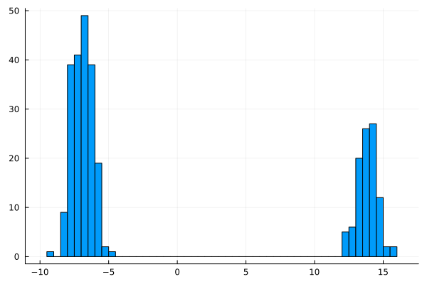
It looks promising. We got two separated clusters. But are they connected with our ids?
julia> histogram(t[ids .== 1]; nbins=20, label="1")

julia> histogram!(t[ids .== 0]; nbins=10, label="0")
You can see the produced plot below:
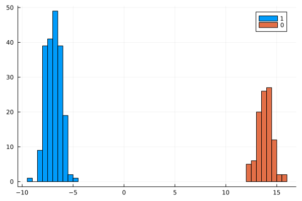
Indeed we got a perfect separation it seems. Let us double check it:
julia> describe(t[ids .== 1])
Summary Stats:
Length:         200
Missing Count:  0
Mean:           -6.914677
Minimum:        -9.086461
1st Quartile:   -7.496597
Median:         -6.926006
3rd Quartile:   -6.359373
Maximum:        -4.606485
Type:           Float64

julia> describe(t[ids .== 0])
Summary Stats:
Length:         100
Missing Count:  0
Mean:           13.829354
Minimum:        12.317402
1st Quartile:   13.322935
Median:         13.911846
3rd Quartile:   14.269240
Maximum:        15.791385
Type:           Float64
The distributions confirm that we recovered the communities correctly.
Conclusions
The presented approach is one of the many that could be used to solve the puzzle. I encourage you to think of alternative approaches that could be used.
However, I think that the puzzle nicely shows that sometimes slightly reformulating the problem allows you to use standard data science tools to solve it.
I hope you enjoyed it!