Some lesser known properties of the coefficient of determination
Introduction
Last week I have posted about p-value in hypothesis testing. I decided to continue discussion of basic statistics today.
My focus will be on computation of Pearson correlation coefficient and the coefficient of determination. I want to concentrate on the fact standard estimators of these quantities are biased.
The post is written under Julia 1.8.5, Distributions 0.25.80, HypergeometricFunctions 0.3.11, HypothesisTests.jl 0.10.11, and Plots.jl 1.38.2.
Testing for bias
In the post we will assume that we have an n-element sample x and y of
two random variables that are normally distributed.
The standard formula for Pearson correlation coefficient between x and y
is (using Julia as pseudocode):
sum(((xi, yi),) -> (xi-mean(x))*(yi-mean(y)), zip(x, y)) /
sqrt(sum(xi -> (xi-mean(x))^2, x) * sum(yi -> (yi-mean(y))^2, y))
Now assume that we want to build a simple linear regression model
where we explain y by x. In this case the coefficient of determination of
this regression is known to be a square of Pearson correlation coefficient
between y and x.
An interesting feature is that both Pearson correlation coefficient and the
coefficient of determination defined above are biased estimators. Let us check
this using a simple experiment. We will generate data for n=10 and true
Pearson correlation between x and y set to 0.5 (note that then the
true coefficient of determination is equal to 0.25).
julia> using Distributions

julia> using Statistics

julia> using Random

julia> function sim(n, ρ)
           dist = MvNormal([1.0 ρ; ρ 1.0])
           x, y = eachrow(rand(dist, n))
           return cor(x, y)
       end
sim (generic function with 1 method)

julia> Random.seed!(1);

julia> cor_sim = [sim(10, 0.5) for _ in 1:10^6];

julia> r2_sim = cor_sim .^ 2;
Now check that the obtained estimators are biased indeed:
julia> using HypothesisTests

julia> OneSampleTTest(cor_sim, 0.5)
One sample t-test
-----------------
Population details:
    parameter of interest:   Mean
    value under h_0:         0.5
    point estimate:          0.478612
    95% confidence interval: (0.4781, 0.4791)

Test summary:
    outcome with 95% confidence: reject h_0
    two-sided p-value:           <1e-99

Details:
    number of observations:   1000000
    t-statistic:              -80.08122936481526
    degrees of freedom:       999999
    empirical standard error: 0.0002670739739448121


julia> OneSampleTTest(r2_sim, 0.25)
One sample t-test
-----------------
Population details:
    parameter of interest:   Mean
    value under h_0:         0.25
    point estimate:          0.300398
    95% confidence interval: (0.3, 0.3008)

Test summary:
    outcome with 95% confidence: reject h_0
    two-sided p-value:           <1e-99

Details:
    number of observations:   1000000
    t-statistic:              231.0430912829669
    degrees of freedom:       999999
    empirical standard error: 0.00021813356867576183
We see a noticeable bias for both coefficients. An interesting feature you might notice is that Pearson correlation coefficient is biased down, while the coefficient of determination is biased up.
Debiasing estimators
Unbiased estimators for our case have been derived over 60 years ago by
Olkin and Pratt. If we denote by r the computed Pearson coefficient
of determination then the unbiased estimates are given using the following
functions:
julia> using HypergeometricFunctions

julia> cor_unbiased(r) = r * _₂F₁(0.5, 0.5, (n-2)/2, 1-r^2)
cor_unbiased (generic function with 1 method)

julia> r2_unbiased(r) = 1 - (1 - r^2) * _₂F₁(1, 1, n/2, 1-r^2) * (n-3)/(n-2)
r2_unbiased (generic function with 1 method)
Let us check them on our data:
julia> OneSampleTTest(cor_unbiased.(cor_sim), 0.5)
One sample t-test
-----------------
Population details:
    parameter of interest:   Mean
    value under h_0:         0.5
    point estimate:          0.499949
    95% confidence interval: (0.4994, 0.5005)

Test summary:
    outcome with 95% confidence: fail to reject h_0
    two-sided p-value:           0.8529

Details:
    number of observations:   1000000
    t-statistic:              -0.18540252488698106
    degrees of freedom:       999999
    empirical standard error: 0.0002740923081266803


julia> OneSampleTTest(r2_unbiased.(cor_sim), 0.25)
One sample t-test
-----------------
Population details:
    parameter of interest:   Mean
    value under h_0:         0.25
    point estimate:          0.249932
    95% confidence interval: (0.2494, 0.2505)

Test summary:
    outcome with 95% confidence: fail to reject h_0
    two-sided p-value:           0.8054

Details:
    number of observations:   1000000
    t-statistic:              -0.24635861593453004
    degrees of freedom:       999999
    empirical standard error: 0.0002750802967082336
Indeed, debiasing worked.
Difference between estimators
Now check the direction of the difference between estimators as a function of
the observed Pearson correlation coefficient (keeping n=10 fixed as above):
julia> using Plots

julia> plot(r -> r - cor_unbiased(r), xlim=[-1, 1], label="r difference",
            xlab="observed r")

julia> plot!(r -> r^2 - r2_unbiased(r), label="r² difference")
You should get the following plot:
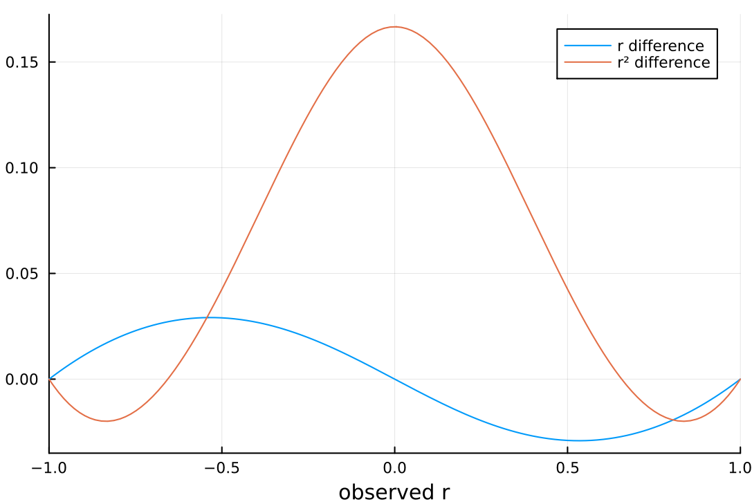
As you can see, Pearson correlation coefficient is always bumped up for positive correlations and down for negative correlations in our case.
Interestingly the coefficient of determination is bumped down if the absolute value of true correlation is less than approximately 0.6565, and if this absolute value is larger then it will be changed up.
This means that we can expect that for large true Pearson coefficient of correlation the standard formula for computing the coefficient of determination will lead to underestimation of the true value on the average.
To check this let us run our simulation again with true r=0.9 and still
keeping n=10:
julia> r2_sim_2 = [sim(10, 0.9)^2 for _ in 1:10^6];

julia> OneSampleTTest(r2_sim_2, 0.81)
One sample t-test
-----------------
Population details:
    parameter of interest:   Mean
    value under h_0:         0.81
    point estimate:          0.796659
    95% confidence interval: (0.7964, 0.7969)

Test summary:
    outcome with 95% confidence: reject h_0
    two-sided p-value:           <1e-99

Details:
    number of observations:   1000000
    t-statistic:              -100.77325436105275
    degrees of freedom:       999999
    empirical standard error: 0.00013238294244740913

julia> OneSampleTTest(r2_unbiased.(sqrt.(r2_sim_2)), 0.81)
One sample t-test
-----------------
Population details:
    parameter of interest:   Mean
    value under h_0:         0.81
    point estimate:          0.810047
    95% confidence interval: (0.8098, 0.8103)

Test summary:
    outcome with 95% confidence: fail to reject h_0
    two-sided p-value:           0.7251

Details:
    number of observations:   1000000
    t-statistic:              0.351680959027248
    degrees of freedom:       999999
    empirical standard error: 0.0001342944339289557
Indeed the coefficient of determination is negatively biased in this case and using Olkin and Pratt method worked again.
So what are the downsides of Olkin and Pratt estimator of the coefficient of
determination? The problem is that it gives negative values for the coefficient
for observed r close to 0. Why is this unavoidable? To see this assume for
a moment that true r=0. In random a sample we will see some positive observed
r^2, just by pure chance. Therefore, to keep the estimator unbiased (note that
its expected value should be 0) we have to allow for its negative values.
Conclusions
I hope you found the presented properties of estimators useful. I think it is quite interesting that even basic statistical methods have quite complex properties, that are not obvious initially.