Metadata in DataFrames.jl: why and how?
Introduction
In my recent post I have discussed new features added in DataFrames.jl. One of them is handling of metadata. Today I want to discuss in more detail why metadata is useful in practice and how it is supported. I am going to cover the following topics:
- Why having metadata support is useful.
- Reading and writing data frames with metadata to disk.
- Rules of metadata propagation.
This post uses many features of data management ecosystem of Julia, so the list of its dependencies is long. I used:
- Julia 1.8.2
- CSV.jl 0.10.7
- DataFrames.jl 1.4.3
- Parquet2.jl 0.2.2
- Plots.jl 1.36.6
- ReadStatTables.jl 0.2.0
- StatsBase.jl 0.33.21
- TableMetadataTools.jl @ 9ce81f87
- ZipFile.jl 0.10.1
Note that the TableMetadataTools.jl package is still in experimental phase, where we are waiting for users’ feedback about its functionality. That is why it is not released yet, and its state is indicated by Git hash:
(@v1.8) pkg> st TableMetadataTools
Status `C:\Users\bogum\.julia\environments\v1.8\Project.toml`
  [9ce81f87] TableMetadataTools v0.1.0
  `https://github.com/JuliaData/TableMetadataTools.jl#main`
Before we start load all the required packages:
julia> using CSV

julia> using DataFrames

julia> import Downloads

julia> using Parquet2

julia> using Plots

julia> import ReadStatTables

julia> using TableMetadataTools

julia> using Serialization

julia> using StatsBase

julia> using ZipFile
The task
The problem for today is to create a plot how percentage of health expenditures in GDP of the United States of America changed over several years.
Assume someone told you that this information can be found in World Bank’s World Development Indicators dataset that is available on this website.
In the post I will follow all the steps that are needed to make the plot.
Getting the data
We first fetch the data and decompress the file storing it:
julia> WDI_URL = "https://sites.google.com/site/md4stata/linked/\
                  world-bank-s-world-development-indicators-wdi/\
                  WDI2009.zip";

julia> if !isfile("WDI2009.dta")
           isfile("WDI2009.zip") || Downloads.download(WDI_URL, "WDI2009.zip");
           zip = ZipFile.Reader("WDI2009.zip")
           open("WDI2009.dta", "w") do io
               write(io, read(only(zip.files)))
           end
           close(zip)
       end
Note that in the code I download and decompress the data only if it is needed.
As a result of our operation we have written to disk the WDI2009.dta file
with the data. The file is in Stata format.
Loading the data into a data frame and inspecting it
julia> df = "WDI2009.dta" |> ReadStatTables.readstat |> DataFrame
11123×872 DataFrame
   Row │ country   wbcode  year   AG_AGR_TRAC_NO  AG_CON_FERT_MT  AG_CON_FER ⋯
       │ String    String  Int16  Float64?        Float64?        Float64?   ⋯
───────┼──────────────────────────────────────────────────────────────────────
     1 │ Aruba     ABW      1960       missing         missing       missing ⋯
     2 │ Aruba     ABW      1961       missing         missing       missing
     3 │ Aruba     ABW      1962       missing         missing       missing
     4 │ Aruba     ABW      1963       missing         missing       missing
     5 │ Aruba     ABW      1964       missing         missing       missing ⋯
     6 │ Aruba     ABW      1965       missing         missing       missing
   ⋮   │    ⋮        ⋮       ⋮          ⋮               ⋮               ⋮    ⋱
 11118 │ Zimbabwe  ZWE      2003         24000.0        146032.0         453
 11119 │ Zimbabwe  ZWE      2004         24000.0         86352.0         268
 11120 │ Zimbabwe  ZWE      2005         24000.0         85018.0         264 ⋯
 11121 │ Zimbabwe  ZWE      2006         24000.0        132661.0     missing
 11122 │ Zimbabwe  ZWE      2007       missing         missing       missing
 11123 │ Zimbabwe  ZWE      2008       missing         missing       missing
                                            867 columns and 11111 rows omitted

julia> describe(df, :min, :max, :nmissing)
872×4 DataFrame
 Row │ variable           min          max         nmissing
     │ Symbol             Any          Any         Int64
─────┼──────────────────────────────────────────────────────
   1 │ country            Afghanistan  Zimbabwe           0
   2 │ wbcode             ABW          ZWE                0
   3 │ year               1960         2008               0
   4 │ AG_AGR_TRAC_NO     1.0          2.79193e7       2294
   5 │ AG_CON_FERT_MT     0.0          5.59256e7       3755
   6 │ AG_CON_FERT_ZS     0.0          1.57833e5       3295
  ⋮  │         ⋮               ⋮           ⋮          ⋮
 867 │ TX_VAL_OTHR_ZS_WT  -3.84e-13    100.0           5792
 868 │ TX_VAL_SERV_CD_WT  0.0          3.81092e12      5713
 869 │ TX_VAL_TECH_CD     0.0          1.80719e12      8696
 870 │ TX_VAL_TECH_MF_ZS  0.0          74.9541         8574
 871 │ TX_VAL_TRAN_ZS_WT  0.000332059  100.0           5938
 872 │ TX_VAL_TRVL_ZS_WT  0.113351     100.0           5913
                                            860 rows omitted
We note that the data set is quite wide. It has almost 900 columns. Additionally we see that column names are not very informative.
This is a common situation when working with wide tables. Authors of such datasets typically try to use relatively short variable names.
How can we find the column that represents percentage of health expenditures in GDP of the United States of America? We clearly need metadata for this table.
Fortunately it is present in this dataset, so let us investigate it. Before we start let me highlight that there are two types of metadata in DataFrames.jl:
- table-level metadata: key-value pairs that are attached to a data frame as a whole; keys must be strings, and values can be arbitrary data (but it is recommended to use strings if interoperability is important, as some storage formats are only able to store string values);
- column-level metadata: key-value pairs that are attached to a concrete column in a data frame (the same considerations about data types of keys and values apply as for table-level metadata).
First check table-level metadata:
julia> metadata(df)
Dict{String, Any} with 13 entries:
  "file_ext"             => ".dta"
  "modified_time"        => DateTime("2010-01-08T11:17:00")
  "file_format_version"  => 114
  "file_format_is_64bit" => false
  "table_name"           => ""
  "notes"                => ["2", "dataset coded for stata as in Catini, Pani…
  "file_encoding"        => ""
  "file_label"           => ""
  "var_count"            => 872
  "row_count"            => 11123
  "creation_time"        => DateTime("2010-01-08T11:17:00")
  "endianness"           => READSTAT_ENDIAN_LITTLE
  "compression"          => READSTAT_COMPRESS_NONE

julia> metadata(df, "notes")
3-element Vector{String}:
 "2"
 "dataset coded for stata as in Catini, Panizza and Saade. Macro Data 4 Stata"
 "December 2009"
We can see that the data set was created on Jan 9, 2010 by Catini, Panizza and Saade in Macro Data 4 Stata project. We also have information that the data frame should have 11123 rows and 872 columns, and indeed above we see that this information is consistent.
Let me comment here on one important distinction:
- metadata such as
"var_countor"row_count"is volatile; most likely transformation of thedfdata frame will invalidate it; - metadata such as
"notes"most likely will not be invalidated whendfis transformed.
DataFrames.jl distinguishes these both scenarios and I discuss how it is done below.
Now check column-level metadata:
julia> colmetadata(df)
Dict{Symbol, Dict{String, Any}} with 872 entries:
  :GC_XPN_OTHR_ZS       => Dict("label"=>"Other expense (% of expense)", "for…
  :SH_DYN_AIDS_ZS       => Dict("label"=>"Prevalence of HIV, total (% of popu…
  :EP_PMP_DESL_CD       => Dict("label"=>"Pump price for diesel fuel (US\$ pe…
  :SL_TLF_PRIM_ZS       => Dict("label"=>"Labor force with primary education …
  :NE_CON_PRVT_PC_KD_ZG => Dict("label"=>"Household final consumption expendi…
  :PA_NUS_PPP           => Dict("label"=>"PPP conversion factor, GDP (LCU per…
  :DT_NFL_WFPG_CD       => Dict("label"=>"UN net multilateral flows, WFP (cur…
  :AG_LND_CREL_HA       => Dict("label"=>"Land under cereal production (hecta…
  :EE_BOD_TOTL_KG       => Dict("label"=>"Organic water pollutant (BOD) emiss…
  :SH_DYN_CHLD_MA       => Dict("label"=>"Mortality rate, male child (per 1,0…
  :ER_LND_PTLD_ZS       => Dict("label"=>"Nationally protected areas (% of to…
  :IP_JRN_ARTC_SC       => Dict("label"=>"Scientific and technical journal ar…
  :NY_GDP_DEFL_KD_ZG    => Dict("label"=>"Inflation, GDP deflator (annual %)"…
  :IT_NET_SECR_P6       => Dict("label"=>"Secure Internet servers (per 1 mill…
  :SE_SEC_ENRL_FE_ZS    => Dict("label"=>"Secondary education, pupils (% fema…
  :FR_INR_LNDP          => Dict("label"=>"Interest rate spread (lending rate …
  ⋮                     => ⋮

julia> colmetadata(df, :country)
Dict{String, Any} with 8 entries:
  "label"         => "CountryName"
  "format"        => "%44s"
  "display_width" => 44
  "measure"       => READSTAT_MEASURE_UNKNOWN
  "alignment"     => READSTAT_ALIGNMENT_RIGHT
  "type"          => READSTAT_TYPE_STRING
  "storage_width" => 0x000000000000002d
  "vallabel"      => Symbol("")
As you can see there is a lot of metadata for each column, but most of it is
technical (and most likely volatile) except for "label" which gives us useful
information about the interpretation of data in the column (and this information
is not invalidated under simple operations on a data frame like dropping rows
or columns).
TableMetadataTools.jl provides a convenience functions label and labels that
extract "label" metadata from a column and all columns respectively:
julia> label(df, :country)
"CountryName"

julia> labels(df)
872-element Vector{String}:
 "CountryName"
 ""
 ""
 "Agricultural machinery, tractors"
 "Fertilizer consumption (metric tons)"
 "Fertilizer consumption (100 grams per hectare of arable land)"
 "Agricultural land (sq. km)"
 "Agricultural land (% of land area)"
 ⋮
 "Merchandise exports (current US\$)"
 "Export value index (2000 = 100)"
 "Computer, communications and other services (% of commercial service exports)"
 "Commercial service exports (current US\$)"
 "High-technology exports (current US\$)"
 "High-technology exports (% of manufactured exports)"
 "Transport services (% of commercial service exports)"
 "Travel services (% of commercial service exports)"
Now we could search in the vector returned by labels for a column containing
information about percentage of health expenditures in GDP. The easiest way
to do it is to use the findlabels function from TableMetadataTools.jl:
julia> findlabels(contains(r"health"i), df)
11-element Vector{Pair{Symbol, String}}:
    :SH_MED_CMHW_P3 => "Community health workers (per 1,000 people)"
    :SH_STA_ARIC_ZS => "ARI treatment (% of children under 5 taken to a health provider)"
    :SH_STA_BRTC_ZS => "Births attended by skilled health staff (% of total)"
    :SH_XPD_EXTR_ZS => "External resources for health (% of total expenditure on health)"
    :SH_XPD_OOPC_ZS => "Out-of-pocket health expenditure (% of private expenditure on health)"
       :SH_XPD_PCAP => "Health expenditure per capita (current US\$)"
    :SH_XPD_PRIV_ZS => "Health expenditure, private (% of GDP)"
       :SH_XPD_PUBL => "Health expenditure, public (% of total health expenditure)"
 :SH_XPD_PUBL_GX_ZS => "Health expenditure, public (% of government expenditure)"
    :SH_XPD_PUBL_ZS => "Health expenditure, public (% of GDP)"
    :SH_XPD_TOTL_ZS => "Health expenditure, total (% of GDP)"
We can see that there are 11 columns whose metadata contains health substring
(case insensitive). Now we can relatively easily find that the column we are
interested in is :SH_XPD_TOTL_ZS:
julia> label(df, :SH_XPD_TOTL_ZS)
"Health expenditure, total (% of GDP)"
Let us inspect it:
julia> df.SH_XPD_TOTL_ZS
11123-element Vector{Union{Missing, Float64}}:
  missing
  missing
  missing
  missing
  missing
  missing
  missing
  missing
 ⋮
  missing
 8.1
 7.6
 8.4
 8.9
 9.3
  missing
  missing

julia> describe(df.SH_XPD_TOTL_ZS)
Summary Stats:
Length:         11123
Missing Count:  10098
Mean:           6.310835
Minimum:        1.300000
1st Quartile:   4.550528
Median:         5.900000
3rd Quartile:   7.800000
Maximum:        17.700000
Type:           Union{Missing, Float64}
Understanding metadata styles: part 1
For our analysis we will only need :country, :year, and :SH_XPD_TOTL_ZS
columns. Let us create a data frame holding them:
julia> health_df = select(df, :country, :year, :SH_XPD_TOTL_ZS)
11123×3 DataFrame
   Row │ country   year   SH_XPD_TOTL_ZS
       │ String    Int16  Float64?
───────┼─────────────────────────────────
     1 │ Aruba      1960       missing
     2 │ Aruba      1961       missing
     3 │ Aruba      1962       missing
     4 │ Aruba      1963       missing
     5 │ Aruba      1964       missing
     6 │ Aruba      1965       missing
   ⋮   │    ⋮        ⋮          ⋮
 11118 │ Zimbabwe   2003             7.6
 11119 │ Zimbabwe   2004             8.4
 11120 │ Zimbabwe   2005             8.9
 11121 │ Zimbabwe   2006             9.3
 11122 │ Zimbabwe   2007       missing
 11123 │ Zimbabwe   2008       missing
                       11111 rows omitted
Now check the column-level metadata of this data frame:
julia> colmetadata(health_df)
Dict{Any, Any}()
It is empty. What is the reason for this. We need to go back to df data frame
and check the style of metadata stored there:
julia> colmetadata(df, :country, style=true)
Dict{String, Tuple{Any, Symbol}} with 8 entries:
  "label"         => ("CountryName", :default)
  "format"        => ("%44s", :default)
  "display_width" => (44, :default)
  "measure"       => (READSTAT_MEASURE_UNKNOWN, :default)
  "alignment"     => (READSTAT_ALIGNMENT_RIGHT, :default)
  "type"          => (READSTAT_TYPE_STRING, :default)
  "storage_width" => (0x000000000000002d, :default)
  "vallabel"      => (Symbol(""), :default)
We see that all metadata for :country column their style is :default (we
could check that this style is set for all metadata in df). The :default
style means that metadata is considered volatile, that is it is dropped under
any transformation of df since it could get invalidated. What if we want to
keep column labels? We need to change their style to :note, which indicates
that metadata is safe to be propagated when data frame is transformed. This can
be conveniently done using the setcolmetadatastyle! function from
TableMetadataTools.jl package:
julia> setcolmetadatastyle!(==("label"), df);

julia> colmetadata(df, :country, style=true)
Dict{String, Tuple{Any, Symbol}} with 8 entries:
  "label"         => ("CountryName", :note)
  "format"        => ("%44s", :default)
  "display_width" => (44, :default)
  "measure"       => (READSTAT_MEASURE_UNKNOWN, :default)
  "alignment"     => (READSTAT_ALIGNMENT_RIGHT, :default)
  "type"          => (READSTAT_TYPE_STRING, :default)
  "storage_width" => (0x000000000000002d, :default)
  "vallabel"      => (Symbol(""), :default)

julia> health_df = select(df, :country, :year, :SH_XPD_TOTL_ZS);

julia> colmetadata(health_df)
Dict{Symbol, Dict{String, String}} with 3 entries:
  :year           => Dict("label"=>"")
  :SH_XPD_TOTL_ZS => Dict("label"=>"Health expenditure, total (% of GDP)")
  :country        => Dict("label"=>"CountryName")
Note that the predicate ==("label") selected only "label" metadata and
by default :setcolmetadatastyle! changes the style to :note (the reason is
that most data frame storage formats will produce :default style by default).
We now see that the select operation nicely kept the column labels. However,
we note that for the :year column the label is not nice, as it is an empty
string. We can change it using the label! function:
julia> label!(health_df, :year, "Year");

julia> labels(health_df)
3-element Vector{String}:
 "CountryName"
 "Year"
 "Health expenditure, total (% of GDP)"
The meta2toml function provides a convenient way to dump all table-level and
column-level metadata in TOML format:
julia> print(meta2toml(health_df))
style = true

[colmetadata.SH_XPD_TOTL_ZS]
label = ["Health expenditure, total (% of GDP)", "note"]

[colmetadata.country]
label = ["CountryName", "note"]

[colmetadata.year]
label = ["Year", "note"]

[metadata]

julia> print(meta2toml(health_df, style=false))
style = false

[colmetadata.SH_XPD_TOTL_ZS]
label = "Health expenditure, total (% of GDP)"

[colmetadata.country]
label = "CountryName"

[colmetadata.year]
label = "Year"

[metadata]
The use of this function is twofold. First, you can use it to get human-readable information about data frame metadata. Second use is to make it easy to save metadata to disk.
Storing metadata persistently
Let us start with writing our data frame to a CSV file. Unfortunately CSVs do
not support metadata. One of the workarounds is to save a TOML file with
metadata generated using the meta2toml function along the CSV file. The
benefit of this approach is that both files are human-readable (and editable).
Let us try saving such files and then reading them back:
julia> CSV.write("health.csv", health_df)
"health.csv"

julia> open("healthmeta.toml", "w") do io
           print(io, meta2toml(health_df))
       end

julia> tmp_df = CSV.read("health.csv", DataFrame);

julia> print(meta2toml(tmp_df))
style = true

[colmetadata]

[metadata]

julia> open("healthmeta.toml") do io
           toml2meta!(tmp_df, io)
       end;

julia> print(meta2toml(tmp_df))
style = true

[colmetadata.SH_XPD_TOTL_ZS]
label = ["Health expenditure, total (% of GDP)", "note"]

[colmetadata.country]
label = ["CountryName", "note"]

[colmetadata.year]
label = ["Year", "note"]

[metadata]

julia> isequal(tmp_df, health_df)
true
We indeed see that both the data and metadata are correctly recovered.
Another common data storage format is Parquet. One of the many benefits of
Parquet is that it allows for storing metadata. So let us save healpth_df to
disk and load back a Parquet file:
julia> Parquet2.writefile("health.parquet", health_df)
✏ Parquet2.FileWriter{IOStream}(health.parquet)

julia> tmp2_df = "health.parquet" |> Parquet2.readfile |> DataFrame;

julia> tmp2_df |> meta2toml |> print
style = true

[colmetadata.SH_XPD_TOTL_ZS]
label = ["Health expenditure, total (% of GDP)", "default"]

[colmetadata.country]
label = ["CountryName", "default"]

[colmetadata.year]
label = ["Year", "default"]

[metadata]

julia> isequal(tmp2_df, health_df)
true
All looks good except for metadata style. Unfortunately the limitation of Parquet format is that it does not have a notion of metadata style. We need to set it manually:
julia> setcolmetadatastyle!(==("label"), tmp2_df);

julia> tmp2_df |> meta2toml |> print
style = true

[colmetadata.SH_XPD_TOTL_ZS]
label = ["Health expenditure, total (% of GDP)", "note"]

[colmetadata.country]
label = ["CountryName", "note"]

[colmetadata.year]
label = ["Year", "note"]

[metadata]
Finally let us try serialization, if short-term storage is enough for us:
julia> tmp3_df = deserialize("health.bin");

julia> tmp3_df |> meta2toml |> print
style = true

[colmetadata.SH_XPD_TOTL_ZS]
label = ["Health expenditure, total (% of GDP)", "note"]

[colmetadata.country]
label = ["CountryName", "note"]

[colmetadata.year]
label = ["Year", "note"]

[metadata]

julia> isequal(tmp3_df, health_df)
true
In case of serialization both data and metadata are fully preserved.
Understanding metadata styles: part 2
We already know that :default metadata style is never propagated (except the
copy function and the DataFrame constructor, which produce a full copy of
all data and metadata in a data frame). What are the propagation rules for
:note-style metadata? Let me discuss the most common cases by example.
The first rule is that dropping rows or columns does not invalidate
:note-style metadata:
julia> dropmissing!(health_df)
1025×3 DataFrame
  Row │ country      year   SH_XPD_TOTL_ZS
      │ String       Int16  Float64
──────┼────────────────────────────────────
    1 │ Andorra       2002             7.0
    2 │ Andorra       2003             7.1
    3 │ Andorra       2004             7.1
    4 │ Andorra       2005             7.5
    5 │ Andorra       2006             7.4
    6 │ Afghanistan   2002             8.3
  ⋮   │      ⋮         ⋮          ⋮
 1020 │ Zambia        2006             6.2
 1021 │ Zimbabwe      2002             8.1
 1022 │ Zimbabwe      2003             7.6
 1023 │ Zimbabwe      2004             8.4
 1024 │ Zimbabwe      2005             8.9
 1025 │ Zimbabwe      2006             9.3
                          1013 rows omitted

julia> health_df |> meta2toml |> print
style = true

[colmetadata.SH_XPD_TOTL_ZS]
label = ["Health expenditure, total (% of GDP)", "note"]

[colmetadata.country]
label = ["CountryName", "note"]

[colmetadata.year]
label = ["Year", "note"]

[metadata]
We dropped rows from our data frame using the dropmissing! function and we
see that metadata is not changed.
The second rule is that column renaming does keep metadata. In our table the
:SH_XPD_TOTL_ZS name of the column is not very easy to remember. Let us
change it:
julia> select!(health_df, :country, :year, :SH_XPD_TOTL_ZS => :health2gdp);

julia> health_df |> meta2toml |> print
style = true

[colmetadata.country]
label = ["CountryName", "note"]

[colmetadata.health2gdp]
label = ["Health expenditure, total (% of GDP)", "note"]

[colmetadata.year]
label = ["Year", "note"]

[metadata]
Again we see that :note-style metadata is kept.
The third rule is that if we transform a column and keep its name then also
:note-style metadada is kept:
julia> tmp4_df = transform(health_df, :country => ByRow(uppercase) => :country)
1025×3 DataFrame
  Row │ country      year   health2gdp
      │ String       Int16  Float64
──────┼────────────────────────────────
    1 │ ANDORRA       2002         7.0
    2 │ ANDORRA       2003         7.1
    3 │ ANDORRA       2004         7.1
    4 │ ANDORRA       2005         7.5
    5 │ ANDORRA       2006         7.4
    6 │ AFGHANISTAN   2002         8.3
  ⋮   │      ⋮         ⋮        ⋮
 1020 │ ZAMBIA        2006         6.2
 1021 │ ZIMBABWE      2002         8.1
 1022 │ ZIMBABWE      2003         7.6
 1023 │ ZIMBABWE      2004         8.4
 1024 │ ZIMBABWE      2005         8.9
 1025 │ ZIMBABWE      2006         9.3
                      1013 rows omitted

julia> tmp4_df |> meta2toml |> print
style = true

[colmetadata.country]
label = ["CountryName", "note"]

[colmetadata.health2gdp]
label = ["Health expenditure, total (% of GDP)", "note"]

[colmetadata.year]
label = ["Year", "note"]

[metadata]
The above rule is important to remember. It assumes that the user does not use the same column name to store qualitatively different information. In this case the transformation was just changing country names to uppercase, which did not change the information it carries.
However, if we wanted to change the :health2gdp column from percentages to
proportions we should change its name, and then metadata for this column is
dropped (you could add an appropriate label for this column manually later):
julia> tmp5_df = select(health_df, :country, :year,
                        :health2gdp =>
                        ByRow(x -> x / 100) =>
                        :health2gdp_prop)
1025×3 DataFrame
  Row │ country      year   health2gdp_prop
      │ String       Int16  Float64
──────┼─────────────────────────────────────
    1 │ Andorra       2002            0.07
    2 │ Andorra       2003            0.071
    3 │ Andorra       2004            0.071
    4 │ Andorra       2005            0.075
    5 │ Andorra       2006            0.074
    6 │ Afghanistan   2002            0.083
  ⋮   │      ⋮         ⋮           ⋮
 1020 │ Zambia        2006            0.062
 1021 │ Zimbabwe      2002            0.081
 1022 │ Zimbabwe      2003            0.076
 1023 │ Zimbabwe      2004            0.084
 1024 │ Zimbabwe      2005            0.089
 1025 │ Zimbabwe      2006            0.093
                           1013 rows omitted

julia> tmp5_df |> meta2toml |> print
style = true

[colmetadata.country]
label = ["CountryName", "note"]

[colmetadata.year]
label = ["Year", "note"]

[metadata]
Let me stress this rule again: we changed the meaning of the data in the column
(here by dividing it by 100) so we use another column name to store it. As you
can see metadata was dropped for :healthe2gdp_prop column.
As a side note: not using the same column name for qualitatively different values is a good practice in general, just as not using the same variable name to store different values in a single function.
Now let us change the shape of our data from long to wide:
julia> health_wide = unstack(health_df, :country, :year, :health2gdp)
205×6 DataFrame
 Row │ country               2002      2003      2004      2005      2006
     │ String                Float64?  Float64?  Float64?  Float64?  Float64?
─────┼────────────────────────────────────────────────────────────────────────
   1 │ Andorra                7.0        7.1      7.1       7.5       7.4
   2 │ Afghanistan            8.3        8.5      8.5       9.5       9.2
   3 │ Angola                 2.3        2.6      2.0       1.9       2.6
   4 │ Albania                6.3        6.3      6.8       6.6       6.5
   5 │ United Arab Emirates   3.4        3.2      2.9       2.7       2.5
   6 │ Argentina              8.9        8.3      9.6      10.2      10.1
  ⋮  │          ⋮               ⋮         ⋮         ⋮         ⋮         ⋮
 200 │ World                  9.94274   10.0342   9.92719   9.87598   9.76724
 201 │ Samoa                  4.9        5.1      4.9       4.8       5.0
 202 │ Yemen, Rep.            4.7        5.1      5.0       5.2       4.5
 203 │ South Africa           8.3        8.0      8.0       8.0       8.0
 204 │ Zambia                 6.6        6.6      6.5       6.8       6.2
 205 │ Zimbabwe               8.1        7.6      8.4       8.9       9.3
                                                              193 rows omitted

julia> health_wide |> meta2toml |> print
style = true

[colmetadata.country]
label = ["CountryName", "note"]

[metadata]
Note that the :country column retains its metadata (we have not transformed
it), but all other newly generated columns do not have any metadata.
As a last example let us keep only rows related to United States in our data frame and additionally add caption metadata for this table:
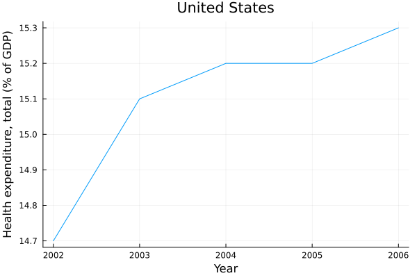
julia> us = health_df[health_df.country .== "United States", :]
5×3 DataFrame
 Row │ country        year   health2gdp
     │ String         Int16  Float64
─────┼──────────────────────────────────
   1 │ United States   2002        14.7
   2 │ United States   2003        15.1
   3 │ United States   2004        15.2
   4 │ United States   2005        15.2
   5 │ United States   2006        15.3

julia> caption!(us, "United States");

julia> us |> meta2toml |> print
style = true

[colmetadata.country]
label = ["CountryName", "note"]

[colmetadata.health2gdp]
label = ["Health expenditure, total (% of GDP)", "note"]

[colmetadata.year]
label = ["Year", "note"]

[metadata]
caption = ["United States", "note"]
We again see that dropping rows keeps :note-style metadata. Also note that
the caption! function creates metadata having :note style.
Plotting the data
We are finally ready to perform the task we were asked to perform. Let us,
using the us data frame, create a plot of how percentage of health
expenditures in GDP of the United States of America changed over several years:
julia> plot(us.year, us.health2gdp,
            xlabel=label(us, :year), ylabel=label(us, :health2gdp),
            title=caption(us), legend=false)
Note that we used table metadata to provide information about axes and title for the plot. By running the above command you should get the following result:
Conclusions
Using metadata in DataFrames.jl makes it easier to organize, find and understand data stored in it.
In this post I mostly concentrated on note metadata (like column labels). As you saw this kind of metadata is useful when you have wide tables (or many tables) to help you easily navigate them.
In general it is possible to manage such metadata in a separate data structure that keeps it outside of data frame object. The benefit of storing metadata within a data frame is that its propagation is automatically handled when data frame is transformed. Therefore DataFrames.jl introduces two styles of metadata:
:defaultstyle: this is meant for metadata that is volatile, and can get invalidated under transformations (in our case number of rows or columns of a data frame were such metadata in the originaldfdata frame);:notestyle: this is meant for metadata that you want to be retained as the data frame is transformed (in our example we wanted to keep column labels).
TableMetadataTools.jl provides convenience methods helping you to perform most common operations on metadata. Of course you can always use DataAPI.jl low-level metadata API if you need a fine-grained control over metadata. TableMetadataTools.jl is still in experimental development phase if you have any comments or feature requests related to it please leave an issue on GitHub.
Apart from various note-like metadata can be useful also in programmatic contexts. Here are some examples:
- GeoDataFrames.jl uses metadata to store information which columns are
geometry columns and about coordinate reference system; note that such
approach has a benefit that this package does not have to create its own data
type; instead it was enough to store metadata information in a data frame
to allow for extra features (this is much easier to do and much cheaper to
maintain - assuming the package likes
DataFrameas an underlying object). - TableMetadataTools.jl provides
@trackmacro. This macro allows you to automatically store in data frame metadata a time-stamped information about all operations that were applied to this data frame. This is a low-overhead method to ensure that you can perform lineage analysis of your data (of course more complicated mechanisms are possible to be implemented, but I wanted to provide something that is as lightweight as possible that does the job). Such functionalities become more and more important in the MLOps and DataOps era.