Pivot tables in DataFrames.jl 1.4
Introduction
Some time ago I have written a post about the unstack function
in DataFrames.jl. Since DataFrames.jl 1.4 release this function has received
a major update of offered functionality. Currently it is possible to
easily create pivot tables using unstack as I am going to show you today.
The example we will use is simulation analysis of graphs, as in May 2023 I am co-organizing 18th Workshop on Algorithms and Models for the Web Graph. If you are interested in this topic please come and join us. If you would like to present your work, here is the Call For Papers.
The post was written under Julia 1.8.2, Graphs.jl 1.7.4, ProgressMeter.jl 1.7.2, Plots.jl 1.36.2, and DataFrames.jl 1.4.3.
Generating the data
We will consider Erdős–Rényi random graphs. These graphs take two
parameters n (the number of nodes in the graph) and p edge probability
(independently for each edge). It can be calculated thus, that the expected
number of edges in this graph is pn(n-1)/2, so expected average node degree
is d=p(n-1). So, given n and d we can calculate p=d/(n-1). In Graphs.jl
you can generate these graphs using the erdos_renyi function.
Connected components of a graph are equivalence classes of a reachability relation between pairs of nodes. Informally: in a connected component all nodes can be reached from each other and no nodes outside from a connected component can be reached from it.
Let me explain it by example:
julia> using Graphs

julia> using Random

julia> Random.seed!(1234);

julia> er = erdos_renyi(7, 0.2)
{7, 4} undirected simple Int64 graph

julia> collect(edges(er))
4-element Vector{Graphs.SimpleGraphs.SimpleEdge{Int64}}:
 Edge 1 => 6
 Edge 3 => 7
 Edge 4 => 6
 Edge 5 => 6

julia> connected_components(er)
3-element Vector{Vector{Int64}}:
 [1, 4, 5, 6]
 [2]
 [3, 7]
We created a random graph on 7 nodes with edge probability equal to 0.2.
It has 4 edges. Note, that our graph is undirected, so although Graphs.jl
displays edges like this: 1 => 6, the edges are bi-directional.
We note that node 6 is connected to nodes 1, 4, and 5. So they
form one connected component. There is also an edge between nodes 3 and 7,
so this is a second connected component. Finally node 2 is isolated, giving
us a third component. We can easily find the connected components of a graph
using the connected_components function.
We will want to investigate how the size of the largest connected component
of the Erdős–Rényi random graph depends on n and d using simulation.
We generate the data for n having values [100, 1000, 10_000, 100_000]
and d having values 0.5:0.1:2.0. For each combination
of values we repeat the experiment 64 times.
First create an initial data frame with the setup of the experiment:
julia> using DataFrames

julia> df = allcombinations(DataFrame,
                            d=0.5:0.1:2.0,
                            n=[100, 1000, 10_000, 100_000],
                            rep=1:64)
4096×3 DataFrame
  Row │ d        n       rep
      │ Float64  Int64   Int64
──────┼────────────────────────
    1 │     0.5     100      1
    2 │     0.6     100      1
    3 │     0.7     100      1
    4 │     0.8     100      1
    5 │     0.9     100      1
  ⋮   │    ⋮       ⋮       ⋮
 4092 │     1.6  100000     64
 4093 │     1.7  100000     64
 4094 │     1.8  100000     64
 4095 │     1.9  100000     64
 4096 │     2.0  100000     64
              4086 rows omitted
Now we compute p for each experiment:
julia> df.p = df.d ./ (df.n .- 1);

julia> df
4096×4 DataFrame
  Row │ d        n       rep    p
      │ Float64  Int64   Int64  Float64
──────┼─────────────────────────────────────
    1 │     0.5     100      1  0.00505051
    2 │     0.6     100      1  0.00606061
    3 │     0.7     100      1  0.00707071
    4 │     0.8     100      1  0.00808081
    5 │     0.9     100      1  0.00909091
  ⋮   │    ⋮       ⋮       ⋮         ⋮
 4092 │     1.6  100000     64  1.60002e-5
 4093 │     1.7  100000     64  1.70002e-5
 4094 │     1.8  100000     64  1.80002e-5
 4095 │     1.9  100000     64  1.90002e-5
 4096 │     2.0  100000     64  2.00002e-5
                           4086 rows omitted
Finally for each row we compute the fraction of nodes in the largest component
(the computation takes some time, so I use @showprogress to monitor it):
julia> using ProgressMeter

julia> df.largest = @showprogress map(eachrow(df)) do row
           er = erdos_renyi(row.n, row.p)
           cc = connected_components(er)
           return maximum(length, cc) / row.n
       end;
Progress: 100%|███████████████████████████████████████████████| Time: 0:00:39

julia> df
4096×5 DataFrame
  Row │ d        n       rep    p            largest
      │ Float64  Int64   Int64  Float64      Float64
──────┼──────────────────────────────────────────────
    1 │     0.5     100      1  0.00505051   0.04
    2 │     0.6     100      1  0.00606061   0.07
    3 │     0.7     100      1  0.00707071   0.22
    4 │     0.8     100      1  0.00808081   0.29
    5 │     0.9     100      1  0.00909091   0.35
  ⋮   │    ⋮       ⋮       ⋮         ⋮          ⋮
 4092 │     1.6  100000     64  1.60002e-5   0.64289
 4093 │     1.7  100000     64  1.70002e-5   0.69333
 4094 │     1.8  100000     64  1.80002e-5   0.73421
 4095 │     1.9  100000     64  1.90002e-5   0.77021
 4096 │     2.0  100000     64  2.00002e-5   0.79805
                                    4086 rows omitted
Now we are ready to analyze this data using unstack.
Analyzing the results
First let me recall the general structure of the unstack call
(please refer to its documentation for more details):
unstack([data_frame],
        [columns to use as row keys],
        [column storing column names],
        [column storing the values];
        combine=[function to apply to the values])
The structure is easy to remember. After a data frame, we sequentially pass
what we want in rows, what we want in columns, what values we want to unstack,
and finally, a combine keyword argument (introduced in DataFrames.jl 1.4)
specifies what operation we want to apply to these values.
By default combine is only, which means that we want a unique value in
row-column combination and otherwise we get an error. Let us check how
unstack works by default by using [:d, :rep] for rows, :n for columns,
and :largest for values:
julia> unstack(df, [:d, :rep], :n, :largest)
1024×6 DataFrame
  Row │ d        rep    100       1000      10000     100000
      │ Float64  Int64  Float64?  Float64?  Float64?  Float64?
──────┼────────────────────────────────────────────────────────
    1 │     0.5      1      0.04     0.009    0.0017   0.00021
    2 │     0.6      1      0.07     0.046    0.0024   0.00035
    3 │     0.7      1      0.22     0.011    0.0042   0.00048
    4 │     0.8      1      0.29     0.019    0.01     0.00139
    5 │     0.9      1      0.35     0.027    0.0109   0.00166
  ⋮   │    ⋮       ⋮       ⋮         ⋮         ⋮         ⋮
 1020 │     1.6     64      0.63     0.665    0.6419   0.64289
 1021 │     1.7     64      0.69     0.683    0.6941   0.69333
 1022 │     1.8     64      0.33     0.746    0.7389   0.73421
 1023 │     1.9     64      0.84     0.761    0.7696   0.77021
 1024 │     2.0     64      0.83     0.818    0.7991   0.79805
                                               1104 rows omitted
Everything worked, because for each cell we had a unique combination of row and
column keys. However, if we, for example, dropped :rep, we would get an
error:
julia> unstack(df, :d, :n, :largest)
ERROR: ArgumentError: Duplicate entries in unstack
at row 65 for key (0.5,) and variable 100.
Pass `combine` keyword argumen t to specify how they should be handled.
Let us start with passing combine=copy to just store all values of
:largest per row-column combination:
julia> unstack(df, :d, :n, :largest, combine=copy)
16×5 DataFrame
 Row │ d        100                                1000
     │ Float64  Array…?                            Array…?
─────┼───────────────────────────────────────────────────────────────────
   1 │     0.5  [0.04, 0.06, 0.05, 0.05, 0.08, 0…  [0.009, 0.015, 0.009,
   2 │     0.6  [0.07, 0.07, 0.05, 0.07, 0.04, 0…  [0.046, 0.013, 0.018,
   3 │     0.7  [0.22, 0.13, 0.05, 0.09, 0.18, 0…  [0.011, 0.019, 0.024,
   4 │     0.8  [0.29, 0.11, 0.08, 0.09, 0.1, 0.…  [0.019, 0.068, 0.018,
   5 │     0.9  [0.35, 0.19, 0.19, 0.19, 0.11, 0…  [0.027, 0.029, 0.057,
   6 │     1.0  [0.42, 0.12, 0.15, 0.22, 0.16, 0…  [0.11, 0.068, 0.042,
   7 │     1.1  [0.26, 0.32, 0.23, 0.69, 0.36, 0…  [0.146, 0.085, 0.266,
   8 │     1.2  [0.45, 0.09, 0.35, 0.42, 0.25, 0…  [0.232, 0.175, 0.338,
   9 │     1.3  [0.49, 0.47, 0.12, 0.17, 0.67, 0…  [0.376, 0.504, 0.434,
  10 │     1.4  [0.36, 0.45, 0.49, 0.49, 0.47, 0…  [0.448, 0.527, 0.443,
  11 │     1.5  [0.72, 0.6, 0.65, 0.57, 0.69, 0.…  [0.577, 0.474, 0.581,
  12 │     1.6  [0.31, 0.77, 0.41, 0.42, 0.73, 0…  [0.639, 0.584, 0.644,
  13 │     1.7  [0.78, 0.62, 0.68, 0.7, 0.67, 0.…  [0.673, 0.651, 0.653,
  14 │     1.8  [0.86, 0.91, 0.7, 0.71, 0.76, 0.…  [0.721, 0.739, 0.748,
  15 │     1.9  [0.8, 0.76, 0.79, 0.83, 0.76, 0.…  [0.791, 0.794, 0.82,
  16 │     2.0  [0.7, 0.74, 0.87, 0.88, 0.83, 0.…  [0.809, 0.776, 0.792,
                                                        3 columns omitted
Sometimes such operation is useful, but often we are interested in some aggregates.
First let us check if indeed the data was generated correctly, i.e. if the
grid indeed has 64 experiments per combination of parameters. For this we use
the combine=length keyword argument (as we just want to check the number
of elements per d-n combination:
julia> unstack(df, :d, :n, :largest, combine=length)
16×5 DataFrame
 Row │ d        100     1000    10000   100000
     │ Float64  Int64?  Int64?  Int64?  Int64?
─────┼─────────────────────────────────────────
   1 │     0.5      64      64      64      64
   2 │     0.6      64      64      64      64
   3 │     0.7      64      64      64      64
   4 │     0.8      64      64      64      64
   5 │     0.9      64      64      64      64
   6 │     1.0      64      64      64      64
   7 │     1.1      64      64      64      64
   8 │     1.2      64      64      64      64
   9 │     1.3      64      64      64      64
  10 │     1.4      64      64      64      64
  11 │     1.5      64      64      64      64
  12 │     1.6      64      64      64      64
  13 │     1.7      64      64      64      64
  14 │     1.8      64      64      64      64
  15 │     1.9      64      64      64      64
  16 │     2.0      64      64      64      64
All looks good. So now we can check the mean and standard deviation of size of the largest connected component for each combination:
julia> using Statistics

julia> unstack(df, :d, :n, :largest, combine=mean)
16×5 DataFrame
 Row │ d        100        1000       10000       100000
     │ Float64  Float64?   Float64?   Float64?    Float64?
─────┼────────────────────────────────────────────────────────
   1 │     0.5  0.0525     0.0109375  0.00178125  0.000269219
   2 │     0.6  0.0776562  0.0159844  0.00266563  0.00040125
   3 │     0.7  0.0982813  0.0222969  0.00409688  0.000635625
   4 │     0.8  0.134375   0.031875   0.00668906  0.00121281
   5 │     0.9  0.161562   0.0485625  0.0136969   0.00312172
   6 │     1.0  0.205937   0.0905312  0.0445984   0.0187338
   7 │     1.1  0.265781   0.150547   0.149169    0.175325
   8 │     1.2  0.355625   0.272266   0.307183    0.313707
   9 │     1.3  0.375156   0.403047   0.421645    0.423478
  10 │     1.4  0.455313   0.503437   0.507891    0.510792
  11 │     1.5  0.594062   0.57925    0.580353    0.582628
  12 │     1.6  0.596719   0.63575    0.6428      0.641092
  13 │     1.7  0.697656   0.689906   0.691744    0.691409
  14 │     1.8  0.738281   0.730672   0.732986    0.732874
  15 │     1.9  0.76125    0.763125   0.768134    0.767024
  16 │     2.0  0.8025     0.797609   0.796216    0.796993

julia> agg_std = unstack(df, :d, :n, :largest, combine=std)
16×5 DataFrame
 Row │ d        100        1000        10000        100000
     │ Float64  Float64?   Float64?    Float64?     Float64?
─────┼──────────────────────────────────────────────────────────
   1 │     0.5  0.0184305  0.00263598  0.000366829  4.57843e-5
   2 │     0.6  0.0422292  0.00599071  0.000623411  8.65108e-5
   3 │     0.7  0.0538238  0.00819539  0.00102446   0.000125444
   4 │     0.8  0.0635928  0.0138844   0.00234887   0.000429261
   5 │     0.9  0.0928426  0.0202656   0.00613093   0.00137704
   6 │     1.0  0.102581   0.0406045   0.026229     0.0111048
   7 │     1.1  0.141442   0.0748327   0.058437     0.0145289
   8 │     1.2  0.15247    0.0863053   0.0289068    0.00968446
   9 │     1.3  0.15323    0.0694691   0.0170002    0.00647732
  10 │     1.4  0.148399   0.0527765   0.0118846    0.00492798
  11 │     1.5  0.118987   0.0439715   0.0121344    0.00403464
  12 │     1.6  0.150407   0.0286661   0.00957977   0.00351468
  13 │     1.7  0.113833   0.0408923   0.00952214   0.00307108
  14 │     1.8  0.0969627  0.021692    0.00890106   0.00240749
  15 │     1.9  0.0829324  0.0224821   0.00788557   0.00210828
  16 │     2.0  0.0755929  0.0213895   0.0066356    0.00233577
What we can notice (I will not go into mathematics of these results; however, if you find such computations interesting please be sure to join us during WAW2023 conference):
- as we increase average node degree the average size of the largest component increases;
- there seems to be a sharp change for average degree above 1; it is especially visible as we increase number of nodes in the graph;
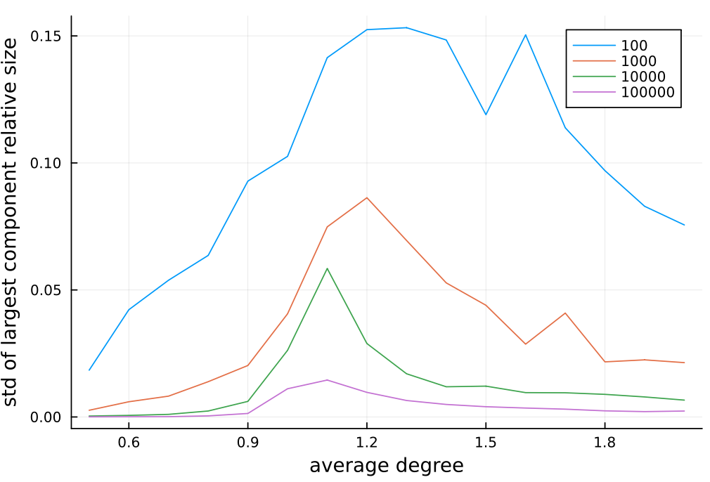
- the results have largest standard deviation around average degree equal to 1; it drops for low and high values of average degree; also the standard deviation in general decreases as we increase number of nodes in the graph.
Let me additionally visualize the last observation:
julia> using Plots

julia> plot(agg_std.d, Matrix(agg_std[:, 2:end]),
            xlabel="average degree",
            ylabel="std of largest component relative size",
            labels=permutedims(names(agg_std, Not(:d))))
Here is a generated plot:
Conclusions
I hope you will find the new combine capabilities of unstack useful.
In DataFrames.jl 1.5 release we plan to add even more capabilities to unstack
(like allowing to use multiple columns to generate columns, or allowing to
process multiple value columns). I will post about it when it is done.