What is the shortest path to AlphaTensor?
Introduction
Recently I have talked with my friend who teaches undergraduate algebra class. We discussed how one can show usefulness of matrix multiplication to students. At the same time a paper about AlphaTensor has been published in nature showing how reinforcement learning was used to discover fast matrix multiplication algorithms.
Trying to combine these two events I thought of a problem where multiplication is much more expensive than addition. You might ask why? Because this condition is required for algorithms like ones discovered by AlphaTensor to be indeed beneficial. One natural candidate is of course multiplication of large matrices, but I wanted something where multiplication of underlying elements of a matrix is much more expensive than their addition. At the same time I wanted a nice example for my friend.
After some thought I decided to use some graph theory. The problem I will write about today is finding shortest paths between all pairs of vertices in a graph. One of the standard algorithms that can be used to perform this task is Floyd–Warshall. Interestingly, the path finding problem can be expressed in terms of matrix multiplication, as is mentioned here. See e.g. chapter 5.9 in “The Design and Analysis of Computer Algorithms” for an introductory explanation.
In this post I will not go into all details of the algorithmic discussion (to leave something for teachers of algebra classes, as it requires giving an introduction to both linear algebra and group theory). Instead, I want to show you, by example, how to compute shortest paths using matrix multiplication and check that indeed we get the expected result. This means that the post today is a bit harder than usual to follow every detail of what I do, but I hope you will still enjoy the narrative.
The presented code was tested under Julia 1.8.2 and Graphs.jl 1.7.4.
Setting up the scene
Let us first generate some test graph and compute distances between all its nodes using Floyd-Warshall algorithm. In the example we will use a well known Zachary’s karate club graph.
julia> using Graphs

julia> g = smallgraph(:karate)
{34, 78} undirected simple Int64 graph

julia> connected_components(g)
1-element Vector{Vector{Int64}}:
 [1, 2, 3, 4, 5, 6, 7, 8, 9, 10  …  25, 26, 27, 28, 29, 30, 31, 32, 33, 34]

julia> g_distances = floyd_warshall_shortest_paths(g).dists
34×34 Matrix{Int64}:
 0  1  1  1  1  1  1  1  1  2  …  2  3  2  2  3  2  1  2  2
 1  0  1  1  2  2  2  1  2  2     3  3  2  2  3  1  2  2  2
 1  1  0  1  2  2  2  1  1  1     3  3  1  1  2  2  2  1  2
 1  1  1  0  2  2  2  1  2  2     3  3  2  2  3  2  2  2  2
 1  2  2  2  0  2  1  2  2  3     3  4  3  3  4  3  2  3  3
 1  2  2  2  2  0  1  2  2  3  …  3  4  3  3  4  3  2  3  3
 ⋮              ⋮              ⋱  ⋮              ⋮
 2  2  1  2  3  3  3  2  2  2     2  2  2  0  2  2  1  2  1
 3  3  2  3  4  4  4  3  2  2     2  1  2  2  0  2  2  1  1
 2  1  2  2  3  3  3  2  1  2  …  3  2  2  2  2  0  2  1  1
 1  2  2  2  2  2  2  2  2  2     1  2  2  1  2  2  0  1  1
 2  2  1  2  3  3  3  2  1  2     2  2  2  2  1  1  1  0  1
 2  2  2  2  3  3  3  3  1  1     2  1  1  1  1  1  1  1  0

julia> maximum(g_distances)
5
Let us look at the plot of the graph:
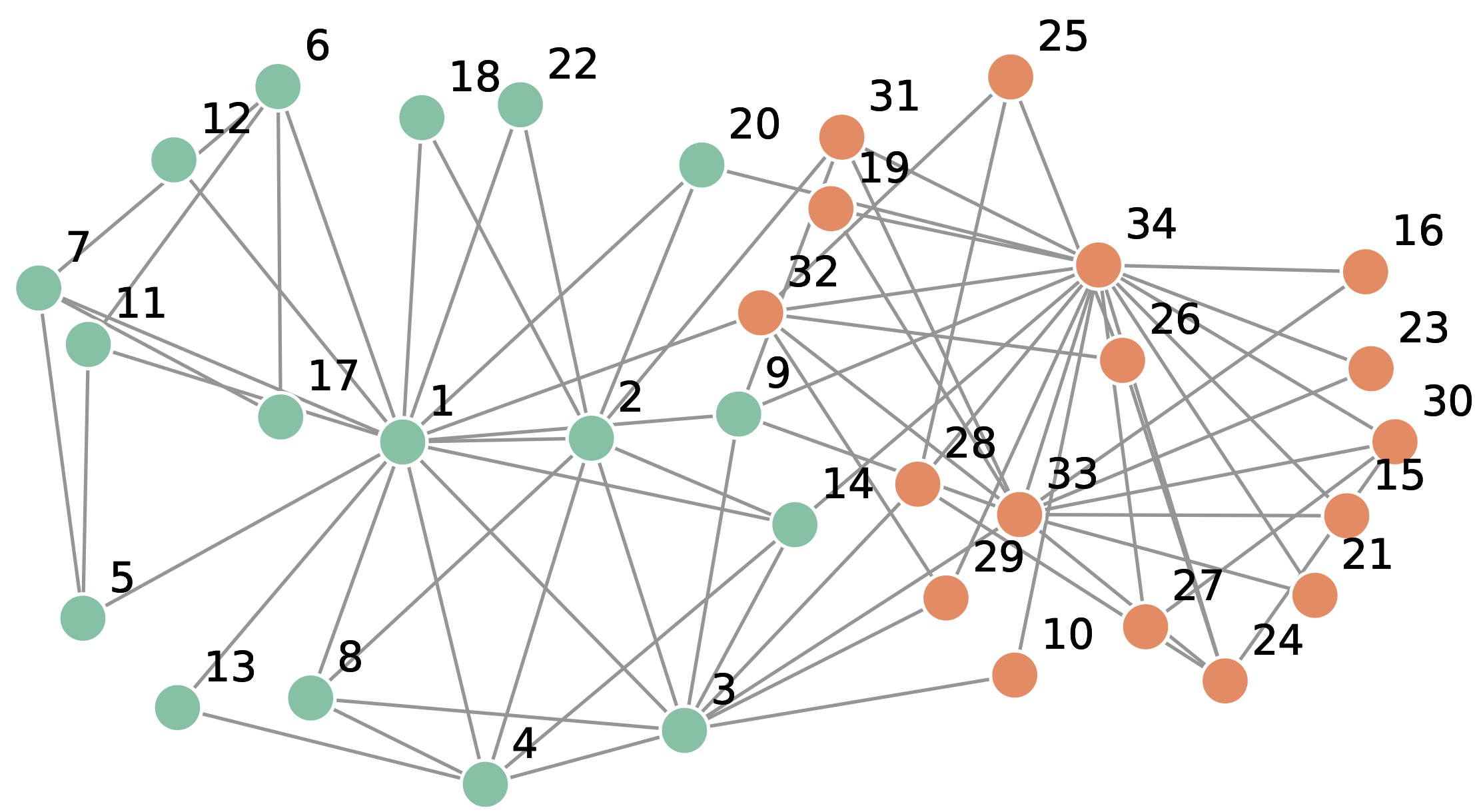
Indeed, we can notice that the graph has one connected component and the biggest distance between two nodes is 5, e.g. between nodes 16 and 17.
We will want now to reproduce the same distances using matrix multiplication and next find the shortest paths also using matrix multiplication.
The first step: distances
To calculate distances let us define Distance type (I make it as simple
as possible to concentrate on matrix multiplication). I supply this type
with custom addition and multiplication definitions that are used for
distance calculation.
julia> struct Distance
           d::Float64
       end

julia> Base.:+(a::Distance, b::Distance) = Distance(min(a.d, b.d))

julia> Base.:*(a::Distance, b::Distance) = Distance(a.d + b.d)

julia> Base.zero(::Distance) = Distance(Inf)

julia> Base.show(io::IO, d::Distance) = show(io, d.d)

julia> Base.float(d::Distance) = d.d
We will start our computations with adjacency matrix, where we put Inf
for nodes that are not connected:
julia> n = nv(g)
34

julia> dm = Distance.([has_edge(g, i, j) ? 1 : i == j ? 0 : Inf
                       for i in 1:n, j in 1:n])
34×34 Matrix{Distance}:
 0.0  1.0  1.0  1.0  1.0  1.0  …  Inf  Inf  1.0  Inf  Inf
 1.0  0.0  1.0  1.0  Inf  Inf     Inf  1.0  Inf  Inf  Inf
 1.0  1.0  0.0  1.0  Inf  Inf     Inf  Inf  Inf  1.0  Inf
 1.0  1.0  1.0  0.0  Inf  Inf     Inf  Inf  Inf  Inf  Inf
 1.0  Inf  Inf  Inf  0.0  Inf     Inf  Inf  Inf  Inf  Inf
 1.0  Inf  Inf  Inf  Inf  0.0  …  Inf  Inf  Inf  Inf  Inf
 ⋮                        ⋮    ⋱       ⋮
 Inf  Inf  1.0  Inf  Inf  Inf     Inf  Inf  1.0  Inf  1.0
 Inf  Inf  Inf  Inf  Inf  Inf     0.0  Inf  Inf  1.0  1.0
 Inf  1.0  Inf  Inf  Inf  Inf  …  Inf  0.0  Inf  1.0  1.0
 1.0  Inf  Inf  Inf  Inf  Inf     Inf  Inf  0.0  1.0  1.0
 Inf  Inf  1.0  Inf  Inf  Inf     1.0  1.0  1.0  0.0  1.0
 Inf  Inf  Inf  Inf  Inf  Inf     1.0  1.0  1.0  1.0  0.0
In the implementation Inf means that at some point we have not yet found
any path between nodes so their distance is infinite.
We are now ready to solve the problem. Since we know that maximal distance in the graph is five, we just can do:
julia> dm^5
34×34 Matrix{Distance}:
 0.0  1.0  1.0  1.0  1.0  1.0  …  3.0  2.0  1.0  2.0  2.0
 1.0  0.0  1.0  1.0  2.0  2.0     3.0  1.0  2.0  2.0  2.0
 1.0  1.0  0.0  1.0  2.0  2.0     2.0  2.0  2.0  1.0  2.0
 1.0  1.0  1.0  0.0  2.0  2.0     3.0  2.0  2.0  2.0  2.0
 1.0  2.0  2.0  2.0  0.0  2.0     4.0  3.0  2.0  3.0  3.0
 1.0  2.0  2.0  2.0  2.0  0.0  …  4.0  3.0  2.0  3.0  3.0
 ⋮                        ⋮    ⋱       ⋮
 2.0  2.0  1.0  2.0  3.0  3.0     2.0  2.0  1.0  2.0  1.0
 3.0  3.0  2.0  3.0  4.0  4.0     0.0  2.0  2.0  1.0  1.0
 2.0  1.0  2.0  2.0  3.0  3.0  …  2.0  0.0  2.0  1.0  1.0
 1.0  2.0  2.0  2.0  2.0  2.0     2.0  2.0  0.0  1.0  1.0
 2.0  2.0  1.0  2.0  3.0  3.0     1.0  1.0  1.0  0.0  1.0
 2.0  2.0  2.0  2.0  3.0  3.0     1.0  1.0  1.0  1.0  0.0
to get the required distances. Let us check:
julia> float.(dm^5) == g_distances
true
Also note that further multiplications of dm do not change anything:
julia> dm^5 == dm^6
true
However, clearly five multiplications are needed:
julia> dm^5 == dm^4
false
In this example addition is min and multiplication is +. Can we do better
and make a bigger difference in cost of these two operations? Yes, we can.
Let us, instead of calculating distances calculate shortest paths.
The final blow: shortest paths
Let us now use the same pattern to compute shortest paths. First define
Path type:
julia> struct Path
           p::Union{Nothing, Vector{Int}}
       end

julia> function Base.:+(a::Path, b::Path)
           isnothing(a.p) && return b
           isnothing(b.p) && return a
           return length(a.p) < length(b.p) ? a : b
       end

julia> function Base.:*(a::Path, b::Path)
           isnothing(a.p) && return Path(nothing)
           isnothing(b.p) && return Path(nothing)
           @assert last(a.p) == first(b.p)
           return Path([a.p; b.p[2:end]])
       end

julia> Base.zero(::Path) = Path(nothing)

julia> Base.show(io::IO, p::Path) = show(io, p.p)

julia> Distance(p::Path) = Distance(isnothing(p.p) ? Inf : length(p.p) - 1)

julia> Base.:(==)(a::Path, b::Path) = a.p == b.p
This time the design is a bit more complex. We denote non-existent path with
nothing. The plus is that clearly multiplication, which involves vector
concatenation, is significantly more expensive than addition (I know it could
be optimized, but I wanted to keep the code simple).
Let us check if indeed still matrix multiplication gives us the desired solution:
julia> pm = [has_edge(g, i, j) ? Path([i, j]) : Path(i == j ? [i] : nothing)
             for i in 1:n, j in 1:n]
34×34 Matrix{Path}:
 [1]      [1, 2]   [1, 3]   [1, 4]   …  nothing   nothing
 [2, 1]   [2]      [2, 3]   [2, 4]      nothing   nothing
 [3, 1]   [3, 2]   [3]      [3, 4]      [3, 33]   nothing
 [4, 1]   [4, 2]   [4, 3]   [4]         nothing   nothing
 [5, 1]   nothing  nothing  nothing     nothing   nothing
 [6, 1]   nothing  nothing  nothing  …  nothing   nothing
 ⋮                                   ⋱
 nothing  nothing  [29, 3]  nothing     nothing   [29, 34]
 nothing  nothing  nothing  nothing     [30, 33]  [30, 34]
 nothing  [31, 2]  nothing  nothing  …  [31, 33]  [31, 34]
 [32, 1]  nothing  nothing  nothing     [32, 33]  [32, 34]
 nothing  nothing  [33, 3]  nothing     [33]      [33, 34]
 nothing  nothing  nothing  nothing     [34, 33]  [34]

julia> pm5 = pm^5
34×34 Matrix{Path}:
 [1]              [1, 2]           …  [1, 32, 34]
 [2, 1]           [2]                 [2, 31, 34]
 [3, 1]           [3, 2]              [3, 33, 34]
 [4, 1]           [4, 2]              [4, 14, 34]
 [5, 1]           [5, 1, 2]           [5, 1, 32, 34]
 [6, 1]           [6, 1, 2]        …  [6, 1, 32, 34]
 ⋮                                 ⋱
 [29, 32, 1]      [29, 3, 2]          [29, 34]
 [30, 34, 32, 1]  [30, 34, 31, 2]     [30, 34]
 [31, 9, 1]       [31, 2]          …  [31, 34]
 [32, 1]          [32, 1, 2]          [32, 34]
 [33, 32, 1]      [33, 31, 2]         [33, 34]
 [34, 32, 1]      [34, 31, 2]         [34]

julia> Distance.(pm5) == dm^5
true

julia> Distance.(pm^6) == dm^5
true

julia> validate(g, p) = all(i -> has_path(g, p.p[i], p.p[i+1]), 1:length(p.p)-1)
validate (generic function with 1 method)

julia> all(p -> validate(g, p), pm5)
true
The validate function checks if indeed some Path is a path in our graph g.
Conclusions
So where is the AlphaTensor stuff in this post? Well - it turns out that it was a click bait. Why cannot we apply AlphaTensor algorithm to our problem? The issue is that it requires the set of values we operate on to be a ring, while the non-standard addition and multiplication we have defined provide only a tropical semiring. Therefore, standard matrix multiplication algorithm works here, as it requires only addition and multiplication. However, AlphaTensor algorithm requires subtraction. So maybe it was not a click bait, but rather an example they one should always check all assumptions of every theorem before using it?
Now let me comment a bit on a Julia side of the examples. I think it is amazing
that everything just worked if we defined custom types with a few extra methods.
Still, there is one thing that might worry you. What if matrix multiplication
algorithm implemented in Base Julia were changed to AlphaTensor or e.g.
Strassen variant (we all know that people behind linear algebra in
Julia are obsessed about performance)? I have a bad and a good news here. The
bad is that we would get an error (and would need to explicitly ask for a
standard multiplication algorithm). Why? Because when subtraction would be
attempted no method to perform it on Distance or Path type would be found.
So what is good news? Well, we would get an error and not an incorrect result,
so we would be explicitly informed that something went wrong.
You might ask why, by default, Julia uses the standard matrix multiplication algorithm? The reason is what we discussed in the introduction. The faster algorithms, like AlphaTensor or Strassen, give benefit only if multiplication is much more expensive than addition. This in practice is encountered for very large matrices. This is not a typical use case against which default linear algebra algorithms in Julia were optimized.
I hope you enjoyed this post! Next week we will go back to discussion of new features introduced in DataFrames.jl 1.4, so stay tuned.