Best kept secret of modern CPU technology

Introduction

When writing complex Julia code we usually want it to run fast. Here the BenchmarkTools.jl package is one of the useful tools that helps developers in writing, running, and comparing benchmark results.

In this post I want to discuss how modern CPUs behave when you benchmark your code by running the same task many times.

In the post I use Julia 1.8.1, BenchmarkTools.jl 1.3.1, and Plots.jl 1.32.1. The machine I used has Intel(R) Core(TM) i7–10850H CPU @ 2.70GHz processor.

Modern CPUs learn the task they are asked to execute

First experiment

Assume we want to benchmark the sum function. Let us run a simple benchmark executing it ten times on a vector having one million elements:

julia> using Plots

julia> using Random

julia> sum(rand(10^6)); # make sure all is compiled

julia> timings_sum(x) = [@elapsed(sum(x)) for i in 1:10]
timings (generic function with 1 method)

julia> plot(timings_sum(rand(10^6));
            legend=false, xlab="run", ylab="time (sec.)")

The result of this test is shown in this plot:

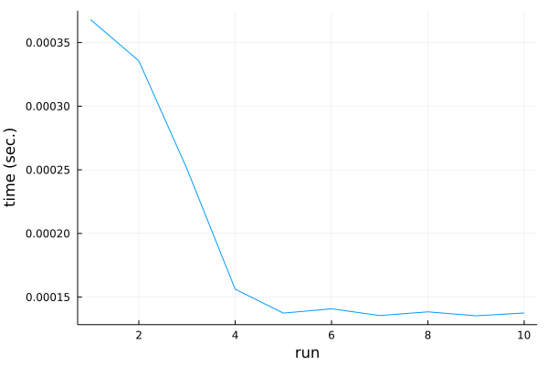
To our surprise the first run of the code is slowest, while consecutive runs are increasingly faster. Things stabilize around fifth run, where code execution time is over two times faster than on the first run.

Is this pattern consistent? Let us run the experiment ten times:

julia> plot([timings_sum(rand(10^6)) for _ in 1:10];
            legend=false, xlab="run", ylab="time (sec.)")

The result is here:

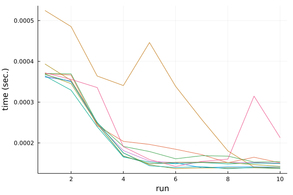
There is some instability, but the general trend is consistent. If we run the sum function repeatedly on the same data it starts to run faster. Allocating a new vector “resets” the performance.

Let us check if the effect is because of new data or new location of the data. This time we keep the same vector, but change data stored in it:

julia> refx = rand(10^6);

julia> plot([timings_sum(rand!(refx)) for _ in 1:10];
            legend=false, xlab="run", ylab="time (sec.)")

The result is here:

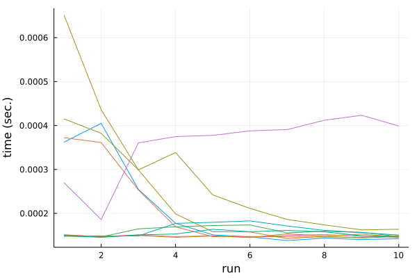
Again there is some instability, but we see that in general it is data location not values of the data that play a role here.

How does it affect the results of using BenchmarkTools.jl? Let us see:

julia> using BenchmarkTools

julia> @btime sum($refx);
  130.500 μs (0 allocations: 0 bytes)

As expected - we get the timing that reflects the performance on old data, not on new data. This is something that we might want. For example, if in our production code we are smart enough not to allocate a new vector every time, but reuse the existing vectors this is a kind of timing that is interesting for us.

However, often we are more interested in timings on new data. This is the way how you can run such benchmark:

julia> b = @benchmarkable sum(benchx) setup=(benchx=rand(10^6))
Benchmark(evals=1, seconds=5.0, samples=10000)

julia> run(b)
BenchmarkTools.Trial: 2221 samples with 1 evaluation.
 Range (min … max):  357.500 μs …   2.022 ms  ┊ GC (min … max): 0.00% … 0.00%
 Time  (median):     372.900 μs               ┊ GC (median):    0.00%
 Time  (mean ± σ):   442.877 μs ± 214.816 μs  ┊ GC (mean ± σ):  0.00% ± 0.00%

  ██▄▁▁  ▂                                                 ▂▁
  █████████▆█▇▇▆▆▅▆▃▄▅▃▃▆▃▃▄▄▁▁▁▁▁▁▃▁▁▁▁▁▁▁▅▄▁▃▃▁▄▄▁▄▃▃▅▅▅███▇▅ █
  358 μs        Histogram: log(frequency) by time       1.22 ms <

 Memory estimate: 0 bytes, allocs estimate: 0.

In this setup note two things. First we use setup to create new data for each sample. Second we do one evaluation per sample. It is important to keep it if we used more evaluations per sample then we would reuse the same vector many times distorting the results:

julia> b.params.evals = 10
10

julia> run(b)
BenchmarkTools.Trial: 1232 samples with 10 evaluations.
 Range (min … max):  187.810 μs … 632.760 μs  ┊ GC (min … max): 0.00% … 0.00%
 Time  (median):     210.325 μs               ┊ GC (median):    0.00%
 Time  (mean ± σ):   226.189 μs ±  55.923 μs  ┊ GC (mean ± σ):  0.00% ± 0.00%

  ▄▆██▇▆▄▄▃▃▂▁▁                                                 ▁
  █████████████▇▇▆▇▆▇██▆▄▁▁▆▄▄▅▁▁▄▁▅▄▅▁▅▅▅▆▄▆▁▁▄▄▆▄▆▅▄▁▄▁▄▁▄▁▁▅ █
  188 μs        Histogram: log(frequency) by time        532 μs <

 Memory estimate: 0 bytes, allocs estimate: 0.

One additional comment is that using 1 evaluation per sample makes sense only if the operation you do is expensive enough to get a proper measurement of its run time (in practice I usually try to benchmark code that is large enough and meets this condition).

Second experiment

Now let us benchmark the findall function on a vector having one million Bool values.

Start with 50% of true and 50% of false:

julia> using Random

julia> findall(trues(10)); # make sure all is compiled

julia> timings_findall(v) = [@elapsed(findall(v)) for i in 1:10]
timings_findall (generic function with 1 method)

julia> x = iseven.(1:1_000_000);

julia> Random.seed!(1234);

julia> y = shuffle(x);

julia> timings_findall(x)
10-element Vector{Float64}:
 0.000711
 0.0007065
 0.0009511
 0.0007604
 0.0007714
 0.0008445
 0.000692
 0.0006092
 0.0078415
 0.0006179

julia> timings_findall(y)
10-element Vector{Float64}:
 0.0007134
 0.0007109
 0.0007077
 0.0006935
 0.0006867
 0.0007165
 0.0007212
 0.0007061
 0.0007018
 0.0007109

julia> @btime findall($x);
  559.900 μs (2 allocations: 3.81 MiB)

julia> @btime findall($y);
  618.900 μs (2 allocations: 3.81 MiB)

We use two vectors. Vector x has true and false in respectively even and odd locations. While vector y is shuffled.

Running timings_findall does not show a strong downward trend like we saw in sum. However, there is some other strange thing happening. Benchmark for vector x runs faster than benchmark for vector y.

Let us re-run the benchmark for the case where we have 1% of true values. Again vector x will have a pattern, while vector y is shuffled:

julia> x = rem.(1:1_000_000, 100) .== 0;

julia> Random.seed!(1234);

julia> y = shuffle(x);

julia> @benchmark findall($x)
BenchmarkTools.Trial: 10000 samples with 1 evaluation.
 Range (min … max):  14.600 μs …  4.553 ms  ┊ GC (min … max):  0.00% … 99.08%
 Time  (median):     19.050 μs              ┊ GC (median):     0.00%
 Time  (mean ± σ):   30.971 μs ± 96.975 μs  ┊ GC (mean ± σ):  10.26% ±  3.41%

  ▂▆██▆▄▃          ▂    ▂▄▄▆▆▇▆▄▃▂           ▁▁               ▃
  ████████▆▅▃▁▁▃▁▅███▇▇█████████████▆▇▆▇▇▆▆▆██████▇▇█████▇▇▆▆ █
  14.6 μs      Histogram: log(frequency) by time      64.1 μs <

 Memory estimate: 78.17 KiB, allocs estimate: 2.

julia> @benchmark findall($y)
BenchmarkTools.Trial: 10000 samples with 1 evaluation.
 Range (min … max):  58.800 μs …  4.784 ms  ┊ GC (min … max): 0.00% … 97.67%
 Time  (median):     66.100 μs              ┊ GC (median):    0.00%
 Time  (mean ± σ):   75.761 μs ± 87.842 μs  ┊ GC (mean ± σ):  3.45% ±  3.18%

  ▆██▇█▆▅▂▁    ▂▅▆▆▇▆▆▅▄▂▁    ▁ ▁▁                            ▃
  ██████████▇██████████████████████▇██▇█▆▇▃▆▅▆▆▆▆▆▅▃▆▅▆▄▆▄▄▅▅ █
  58.8 μs      Histogram: log(frequency) by time       134 μs <

 Memory estimate: 78.17 KiB, allocs estimate: 2.

Now the performance difference is even bigger.

What would happen if we allocated a fresh x vector each time?

julia> b2 = @benchmarkable findall(benchx) setup=(benchx=rem.(1:1_000_000, 100) .== 0)
Benchmark(evals=1, seconds=5.0, samples=10000)

julia> run(b2)
BenchmarkTools.Trial: 5943 samples with 1 evaluation.
 Range (min … max):  14.400 μs …  4.913 ms  ┊ GC (min … max): 0.00% … 99.12%
 Time  (median):     17.800 μs              ┊ GC (median):    0.00%
 Time  (mean ± σ):   26.622 μs ± 86.793 μs  ┊ GC (mean ± σ):  8.59% ±  2.86%

  ▂▅▇█▇▅▃▂              ▁▄▄▅▅▅▄▃▂▁                            ▂
  ███████████▇███▆▆▆▃▅▆▇██████████████▆▇▆▆▆▆▆▄▆▅▆▆▃▄▆▄▅▆▄▆▆▆▆ █
  14.4 μs      Histogram: log(frequency) by time        59 μs <

 Memory estimate: 78.17 KiB, allocs estimate: 2.

We can see that the performance now is comparable. So it is not the issue of new memory location. Now the issue is in the data. My CPU seems to be able to learn that in the vector x the true and false values form a pattern and takes advantage of this when executing my code.

Conclusions

CPUs these days are very smart in how they execute the code. They can do things like RAM caching and branch prediction to improve the run time of your programs. If you would like to read more about such topics then this and this are nice places to check out.

The conclusions from the tests we run today are:

• if your code can be affected by RAM caching make sure to use a proper benchmarking approach that matches the use case in your production code (i.e. either reuse the same data or use setup option and @benchmarkable)
• if your code can be affected by branch prediction make sure that the test data matches your production data (e.g. if in production you expect data that has some structure use a similar structure for testing)

To wrap up I would like to thank Jakob, Kristoffer, Valentin, and Jeffrey for a discussion on this topic on #becnchmarking channel in Julia Slack.