Introduction

It was April 1st, when I was writing my last post, but my friends, after having read it, told me that it was not very funny. So today I get back to boring style.

In the previous post I was comparing lookup speed in vector vs set in Julia and considered a scenario when lookup in vector was faster. This is not something that normally we should expect, but clearly I must have chosen the benchmark settings in a way that lead to such a result.

Today let me go back to that example and discuss it in more detail.

The post was written under Julia 1.7.0, DataFrames.jl 1.3.2, BenchmarkTools.jl 1.3.1, and Plots.jl 1.27.1.

The experiment

Let me remind you the experiment setting. I tested the lookup performance for collections from size 10 to 40. I used random strings and then performed a check if every value stored in the collection is indeed present in it.

Here is the test code I used with one twist. In my original post I have measured total time of lookup. This time I measure time of lookup per single element (the difference is in the plot command where now I divide everything by df.i).

using DataFrames
using BenchmarkTools
using Random
using Plots

f(x, r) = all(in(x), r) # function testing lookup speed

df = DataFrame()
Random.seed!(1234)

for i in 10:40
    v = [randstring(rand(1:1000)) for _ in 1:i] # randomly generate a Vector
    s = Set(v) # turn it to Set for comparison
    @assert length(s) == i # make sure we had no duplicates
    t1 = @belapsed f($s, $v)
    t2 = @belapsed f($v, $v)
    # display the intermetiate results so that I can monitor the progress
    @show (i, t1, t2)
    push!(df, (;i, t1, t2))
end

plot(df.i, [df.t1 df.t2] ./ df.i;
     labels=["Set" "Vector"],
     legend=:topleft,
     xlabel="collection size",
     ylabel="time per lookup in seconds")

The code produces the following plot:

Benchmarks plot 1

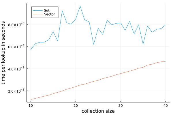
We can see that the lookup time of one element in Set is roughly constant, but for Vector it grows linearly. This is expected. Amortized time of random lookup in Set is O(1) while for Vector it is O(n), where n is collection size.

Last week I have computed total time, which is roughly linear for Set while it is quadratic for Vector. However, I have scaled the plot in a way that it was not very visible that the curve for Vector is a parabola.

Now we can clearly see that we can expect that for larger collections Set will be faster. Let us pick i = 1000 as an example (not very large number, but big enough):

julia> i = 1000;

julia> v = [randstring(rand(1:1000)) for _ in 1:i];

julia> s = Set(v);

julia> @assert length(s) == i

julia> @belapsed f($s, $v)
8.8383e-5

julia> @belapsed f($v, $v)
0.001030348

As you can see now Vector is much slower.

But why was Vector faster than Set for the original data?

Understanding lookup process in `Set` and in `Vector`

When you search for a value in a Set Julia roughly does the following steps:

compute hash of the value you look for;
check if Set contains some values that have the same hash (there might be more than one such value due to collisions);
if yes then check if any of them are equal to the value we have provided.

When you search for a value in a Vector the process is simpler: Julia checks sequentially checks elements of a vector if they are equal to the value you passed. So as you can see the extra cost of using Set is that you need to perform hashing.

In my example I have generated the data using the following expression: [randstring(rand(1:1000)) for _ in 1:i]. As you can see these are random strings that in general can be quite long (up to 1000 characters). Hashing such strings is expensive. The additional trick I did was to generate the strings so that with high probability they have a different length. I did this to make sure that string comparison is fast. As you can check in the implementation of isequal in Julia it falls back to == in this case, which for String is:

function ==(a::String, b::String)
    pointer_from_objref(a) == pointer_from_objref(b) && return true
    al = sizeof(a)
    return al == sizeof(b) && 0 == _memcmp(a, b, al)
end

We can observe that if strings have unequal lengths they are compared very fast.

In summary, I have baked the example so that hashing is expensive but comparison is cheap. If I used shorter strings, e.g. of length 2, then even for i = 10 on the average Set lookup would be faster than Vector lookup:

julia> i = 10;

julia> v = [randstring(2) for _ in 1:i];

julia> s = Set(v);

julia> @assert length(s) == i

julia> @belapsed f($s, $v)
1.47515625e-7

julia> @belapsed f($v, $v)
1.8996439628482973e-7

Of course for very short collections, like e.g. length 1 Set will be slower even in this case as it still would compute hash.

Understanding volatility of `Set` timing

An additional issue that we have noticed last week is smoothness of Vector plot and volatility of Set plot. What is the reason for this? There are two factors here in play:

For each i I use random strings of different lengths. This means that hashing cost differs per experiment. On the other hand for Vector we do not need to do hashing and, as I commented above, we can immediately decide that strings are different just by looking at their length.
For different i Set has different percentage of occupied slots, which means that number of hash collisions that can happen differs.

Conclusions

My takeaways from today’s post are:

benchmarking is useful, but it is important to understand the data structures and algorithms that one uses;
when doing visualization it is really important to think what measures to use so that the plots are informative;
and finally: Set’s not dead (although sometimes indeed it is not an optimal data structure; in general I recommend you to have a look at the options available in DataStructures.jl).

Introduction

The experiment

Understanding lookup process in Set and in Vector

Understanding volatility of Set timing

Conclusions

Understanding lookup process in `Set` and in `Vector`

Understanding volatility of `Set` timing