Introduction

One of the projects I am currently working on is writing the Julia for Data Analysis book. In this post I want to give you a brief overview of the contents of the book and its current status.

What is the objective of the book?

The book is aimed at data scientists with some programming experience wanting to learn how to do data analysis in Julia. Some previous experience with Julia would be a plus, but it is not strictly required.

Since the book is aimed as an entry-level introduction to data analysis in Julia I have divided it into two parts:

Part 1 is teaching you the essential Julia skills you need to learn to confidently use the language.
Part 2 is focused on data analysis.

I do not assume that you know the Julia language and in Part 1 explain the basic components of the language from the very beginning. However, I assume that you have some experience with programming (e.g. in R or Python).

Part 2 focuses on data analysis in Julia. In it I concentrate a lot on the functionalities of the DataFrames.jl package.

It is impossible to cover every aspect of data analysis in Julia in a single book. Therefore, my goal was to discuss all essential material that will allow you to later confidently learn more advanced things on your own, while being convenient that you have a firm grasp of the fundamental concepts.

What is the scope of the book?

Most of the chapters in the book are project oriented. I introduce new concepts and functionalities of the Julia ecosystem by showing how they can be used to solve practical problems.

Since the scope of the book is quite wide let me here list selected technical topics that I discuss in it which, I think, are useful even for people who already know Julia:

working with source data in various formats: CSV, Apache Arrow, SQLite, JSON, serialization, parsing data that has non-standard format;
getting data from external sources (like: downloading data, unpacking compressed data, getting data using HTTP requests, finishing with writing a web service on your own);
solving typical issues encountered when pre-processing data: efficient handling of strings, using categorical values, working with time-series, understanding missing values.
coverage of key functionalities of the DataFrames.jl package and DataFramesMeta.jl package (creating data frames, transforming them, split-apply-combine strategy, joining, sorting, subsetting, reshaping);
creating plots that visualize the results of your analysis using the Plots.jl package;
building simple predictive models (linear regression, logistic regression, LOESS) and assessment of the model performance;
integrating Julia code with R and Python.

Notably, I have not covered in this book more advanced topics on machine learning. The reason is that there are too many options available, so this would be a material for another book. However, as I have already mentioned, the book is written in a way so that after reading it you should be able to easily learn the functionalities of the concrete packages that provide such functionalities, like e.g. MLJ.jl, yourself.

For example, after reading this book you might want to check out my Hands-on Data Science with Julia live project that gives you an introduction to machine learning with Julia.

Where to get the book?

The book will be published by Manning. This week its first two chapters have been made available in MEAP (Manning Early Access Platform).

You can find a preview of the book under this link.

If you are interested in the topic I encourage you to visit the website, as MEAP program gives the readers an opportunity to give feedback about the material I have prepared before the final version of the book is published.

What is the status of the book?

All core chapters have been already written. Now we are going through a review and publishing process. I will write another post when the book is finalized.

However, since all the technical material is already prepared, you can get the source codes of all chapters from GitHub. Codes are shared there are under MIT license so you can freely reuse them.

Conclusions

Today, as a conclusion, let me pick one example code from the book (codes are also available on GitHub).

The example code produces a plot that compares speed and code size of Julia, Python, Java, and C on 10 standard problems taken from the The Computer Language Benchmarks Game website.

The example is self-contained and was tested under Julia 1.7.0, DataFrames.jl 1.3.2, CSV.jl 0.10.3, and Plots.jl 1.27.1.

data = """
problem,language,time,size
n-body,c,2.13,1633
mandelbrot,c,1.3,1135
spectral norm,c,0.41,1197
fannkuch-redux,c,7.58,910
fasta,c,0.78,1463
k-nucleotide,c,3.96,1506
binary-trees,c,1.58,809
reverse-complement,c,0.41,1965
pidigits,c,0.56,1090
regex-redux,c,0.8,1397
n-body,Java,6.77,1489
mandelbrot,Java,4.1,796
spectral norm,Java,1.55,756
fannkuch-redux,Java,10.48,1282
fasta,Java,1.2,2543
k-nucleotide,Java,4.83,1812
binary-trees,Java,2.51,835
reverse-complement,Java,1.57,2183
pidigits,Java,0.79,764
regex-redux,Java,5.34,929
n-body,Python,541.34,1196
mandelbrot,Python,177.35,688
spectral norm,Python,112.97,407
fannkuch-redux,Python,341.45,950
fasta,Python,36.9,1947
k-nucleotide,Python,46.31,1967
binary-trees,Python,44.7,660
reverse-complement,Python,6.62,814
pidigits,Python,1.16,567
regex-redux,Python,1.34,1403
n-body,Julia,4.21,1111
mandelbrot,Julia,1.42,619
spectral norm,Julia,1.11,429
fannkuch-redux,Julia,7.83,1067
fasta,Julia,1.13,1082
k-nucleotide,Julia,4.94,951
binary-trees,Julia,7.28,634
reverse-complement,Julia,1.44,522
pidigits,Julia,0.97,506
regex-redux,Julia,1.74,759
"""

using CSV
using DataFrames
using Plots

df = CSV.read(IOBuffer(data), DataFrame)

plot(map([:time, :size],
         ["execution time (relative to C)",
          "code size (relative to C)"]) do col, title
    df_plot = unstack(df, :problem, :language, col)
    df_plot[!, Not(:problem)] ./= df_plot.c
    select!(df_plot, Not(:c))
    scatter(df_plot.problem, Matrix(select(df_plot, Not(:problem)));
            labels=permutedims(names(df_plot, Not(:problem))),
            ylabel=title,
            yaxis = col == :time ? :log : :none,
            xrotation=20,
            markershape=[:rect :diamond :circle],
            markersize=[4 5 5],
            markercolor=[:lightgray :lightgray :gold],
            xtickfontsize=7, ytickfontsize=7,
            legendfontsize=7, ylabelfontsize=7)
            hline!([1.0]; color="orange", labels="C")
end...)

(the code is not easy, but after reading the whole book you should be able to confidently read it and create a similar implementation yourself)

The figure produced by this code looks as follows.

Benchmarks plot

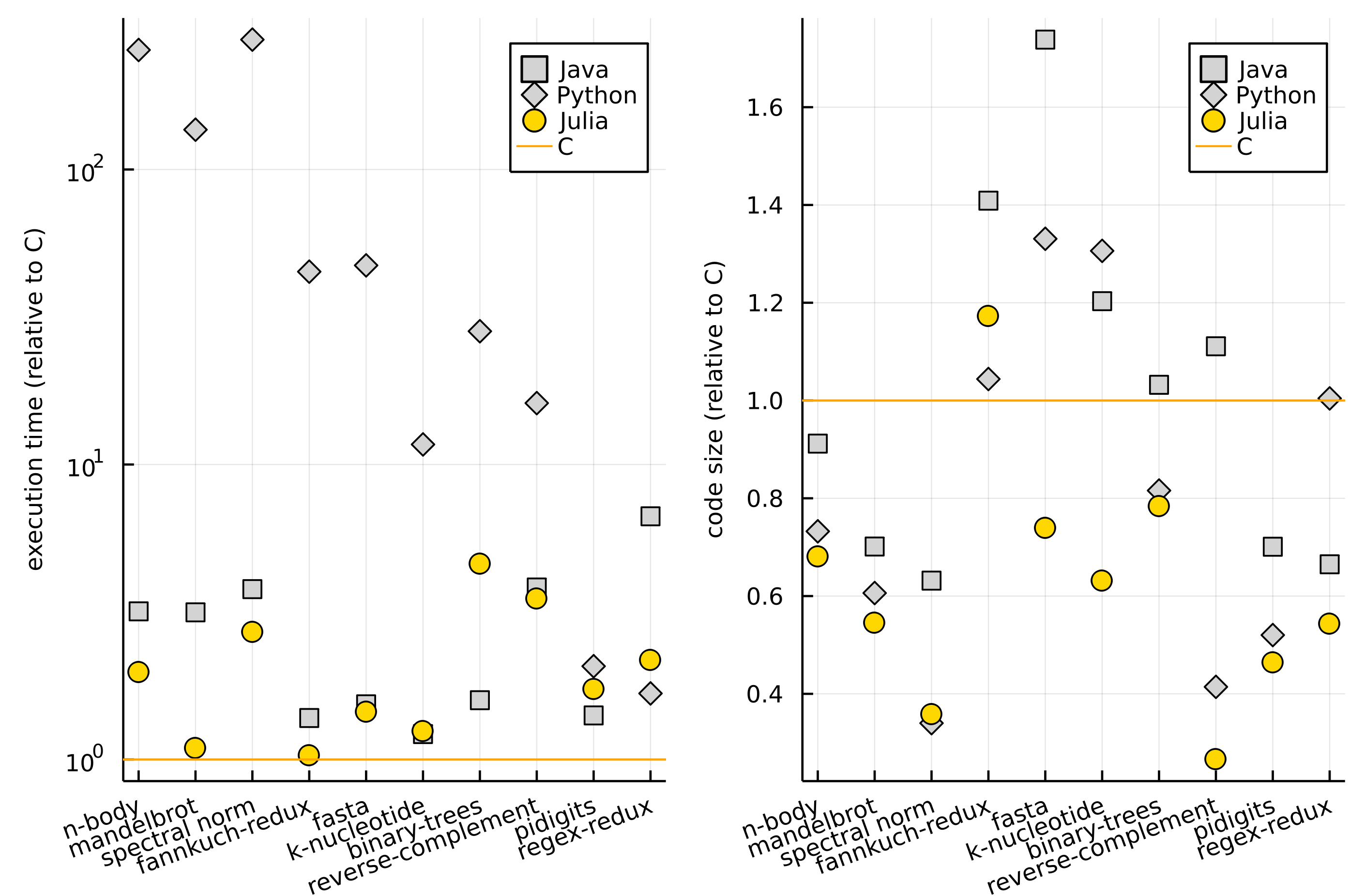
If you would like to read a complete interpretation of the plot please check Chapter 1 in Julia for Data Analysis book. Here let me just summarize that Julia runs the code fast (left pane) and at the same time is convenient to use (as measured by the code size; right pane).