Welcome to DataFramesMeta.jl
Introduction
If you start using Julia for data science you might get overwhelmed by the number of available options and features. Today I want to write about the DataFramesMeta.jl package that greatly simplifies one of the most difficult parts of the DataFrames.jl package to learn, namely - performing data transformations.
In this post I will omit all advanced features of both DataFramesMeta.jl and DataFrames.jl and focus on simple issues to help you build a correct mental model how things should be used.
The post was written under Julia 1.6.3, DataFrames.jl 1.2.2, and DataFramesMeta.jl 0.10.0.
Setting up the stage
Let us first load the required packages and create some simple data frame we will want to work with:
julia> using DataFramesMeta

julia> using Statistics

julia> df = DataFrame(x=1:5, y=11:15)
5×2 DataFrame
 Row │ x      y
     │ Int64  Int64
─────┼──────────────
   1 │     1     11
   2 │     2     12
   3 │     3     13
   4 │     4     14
   5 │     5     15
Notice that when we load DataFramesMeta.jl also DataFrames.jl is automatically loaded to your working environment. Additionally, I have loaded the Statistics module as soon we will use it in our examples.
Understanding data transformations
When you want to perform some transformation of your data the first thing you need to answer is if you want to aggregate data or manipulate columns.
Data aggregation is a simple concept - I take a column as input and produce e.g.
its mean, which is a single aggregated value. In DataFrames.jl we call this
operation combine, as we are combining rows.
When I talk about column manipulation I mean operations that we take a column
and produce output that is also a column that has the same number of elements
as the source, e.g. I multiply the column by 2. In DataFrames.jl we call this
operation either select or transform. What is the difference between
select and transform? When you perform a select operation you keep in the
result only the results of the operations you performed. On the other hand,
when you transform a data frame you additionally keep all the columns from
the source data frame.
Let us now have a look at examples of these three operations. Start with aggregation:
julia> @combine(df, :sum_x = sum(:x), :mean_y = mean(:y))
1×2 DataFrame
 Row │ sum_x  mean_y
     │ Int64  Float64
─────┼────────────────
   1 │    15     13.0
As you can see we used the combine word and prepended it with @ which
signals that this is a DataFramesMeta.jl operation. As a first argument in our
call we passed the source data frame. Next we specified the aggregations we
want to perform. Note that each aggregation is specified just as you would
write normal Julia code using variables. There is only one rule to learn. When
you prefix the variable name with : it means that you are referring to a
column of a data frame.
Now let us perform selection and transformation side by side to see the difference:
julia> @select(df, :z = :x + :y)
5×1 DataFrame
 Row │ z
     │ Int64
─────┼───────
   1 │    12
   2 │    14
   3 │    16
   4 │    18
   5 │    20

julia> @transform(df, :z = :x + :y)
5×3 DataFrame
 Row │ x      y      z
     │ Int64  Int64  Int64
─────┼─────────────────────
   1 │     1     11     12
   2 │     2     12     14
   3 │     3     13     16
   4 │     4     14     18
   5 │     5     15     20
As you can see both operations create a new column :z. The difference is that
@transform also keeps the :x and :y variables, while @select drops them.
Let us write another transformation:
julia> @transform(df, :z = :x * :y)
ERROR: MethodError: no method matching *(::Vector{Int64}, ::Vector{Int64})
This time the operation failed. Most Julia users know why. You cannot multiply a vector by a vector - this is not a properly defined mathematical operation. Instead you have to broadcast the multiplication operation like this (this is often called a vectorized operation):
julia> @transform(df, :z = :x .* :y)
5×3 DataFrame
 Row │ x      y      z
     │ Int64  Int64  Int64
─────┼─────────────────────
   1 │     1     11     11
   2 │     2     12     24
   3 │     3     13     39
   4 │     4     14     56
   5 │     5     15     75
In more complex scenarios adding the . for broadcasting can easily get
annoying, e.g.:
julia> @transform(df, :a = 2 .* :x, :b = :x .* :y .^ 2)
5×4 DataFrame
 Row │ x      y      a      b
     │ Int64  Int64  Int64  Int64
─────┼────────────────────────────
   1 │     1     11      2    121
   2 │     2     12      4    288
   3 │     3     13      6    507
   4 │     4     14      8    784
   5 │     5     15     10   1125
On the other hand practice shows that such broadcasted operations are quite
common. Therefore in DataFrames.jl parlance they are called by-row operations.
DataFramesMeta.jl allows an easy way to tell @select and @transform that
all operations that user passes to them should be applied by-row. Just prefix
the name of the transformation function with the r character (r stands for
row). Therefore we have @rselect and @rtransform:
julia> @rselect(df, :a = 2 * :x, :b = :x * :y ^ 2)
5×2 DataFrame
 Row │ a      b
     │ Int64  Int64
─────┼──────────────
   1 │     2    121
   2 │     4    288
   3 │     6    507
   4 │     8    784
   5 │    10   1125

julia> @rtransform(df, :a = 2 * :x, :b = :x * :y ^ 2)
5×4 DataFrame
 Row │ x      y      a      b
     │ Int64  Int64  Int64  Int64
─────┼────────────────────────────
   1 │     1     11      2    121
   2 │     2     12      4    288
   3 │     3     13      6    507
   4 │     4     14      8    784
   5 │     5     15     10   1125
As you can see we got rid of the dots, paying the cost of having all operations applied by-row to our data.
As an exercise think how you would subtract the mean from column :x in our
data frame. Can we use @rselect or we must use @select? You can use both:
julia> @select(df, :x, :x2 = :x .- mean(:x))
5×2 DataFrame
 Row │ x      x2
     │ Int64  Float64
─────┼────────────────
   1 │     1     -2.0
   2 │     2     -1.0
   3 │     3      0.0
   4 │     4      1.0
   5 │     5      2.0

julia> @rselect(df, :x, :x2 = :x - mean(df.x))
5×2 DataFrame
 Row │ x      x2
     │ Int64  Float64
─────┼────────────────
   1 │     1     -2.0
   2 │     2     -1.0
   3 │     3      0.0
   4 │     4      1.0
   5 │     5      2.0
I would say, however, that this time using @select is more natural. Although
we have to use the . in :x2 = :x .- mean(:x) it is pretty easy to understand
what was going on there. Additionally the @rselect version will be slower as
it will recompute mean(df.x) for each row of the data frame.
When we used @rselect we had to pass the df.x column to the mean (this is a
value computed as any other Julia code, DataFramesMeta.jl does not touch it as
it does not have : in front). Note that just passing :x would be incorrect,
as mean would be also applied by-row to it so we would broadcast mean over
the :x column and the result would be:
julia> @rselect(df, :x, :x2 = :x - mean(:x))
5×2 DataFrame
 Row │ x      x2
     │ Int64  Float64
─────┼────────────────
   1 │     1      0.0
   2 │     2      0.0
   3 │     3      0.0
   4 │     4      0.0
   5 │     5      0.0
and this is most likely not what we want (unless we wanted to check that
subtracting some number from itself is equal to zero). In summary putting a r
prefix broadcasts the operation with respect to the columns of a data frame
(i.e. parts of the passed expression that contain names with a : prefix).
So now we know that if we prefix select or transform with r we switch to
by-row mode. Is there anything more to learn? Indeed there is one more thing
you need to know. This is a ! suffix that these functions can take. What it
does is that it makes the operation update the passed data frame. Note that
above when we performed transformations we were getting a fresh data frame, but
our df source data frame was untouched. When you suffix ! you get exactly
the same result but it gets stored in the data frame you passed to the
operation. Here are some examples:
julia> df
5×2 DataFrame
 Row │ x      y
     │ Int64  Int64
─────┼──────────────
   1 │     1     11
   2 │     2     12
   3 │     3     13
   4 │     4     14
   5 │     5     15

julia> @transform!(df, :z = :x + :y)
5×3 DataFrame
 Row │ x      y      z
     │ Int64  Int64  Int64
─────┼─────────────────────
   1 │     1     11     12
   2 │     2     12     14
   3 │     3     13     16
   4 │     4     14     18
   5 │     5     15     20

julia> df
5×3 DataFrame
 Row │ x      y      z
     │ Int64  Int64  Int64
─────┼─────────────────────
   1 │     1     11     12
   2 │     2     12     14
   3 │     3     13     16
   4 │     4     14     18
   5 │     5     15     20

julia> @select!(df, :s = :x + :y + :z)
5×1 DataFrame
 Row │ s
     │ Int64
─────┼───────
   1 │    24
   2 │    28
   3 │    32
   4 │    36
   5 │    40

julia> df
5×1 DataFrame
 Row │ s
     │ Int64
─────┼───────
   1 │    24
   2 │    28
   3 │    32
   4 │    36
   5 │    40
Why might we want such in-place operations? Consider a large data frame
with 10,000 columns. If you perform a @transform of such a data frame adding
one column to it you will copy a lot of data (which takes time and RAM). By
doing @transform! you will be faster and more memory efficient, at the expense
of mutating the source data frame.
Conclusions
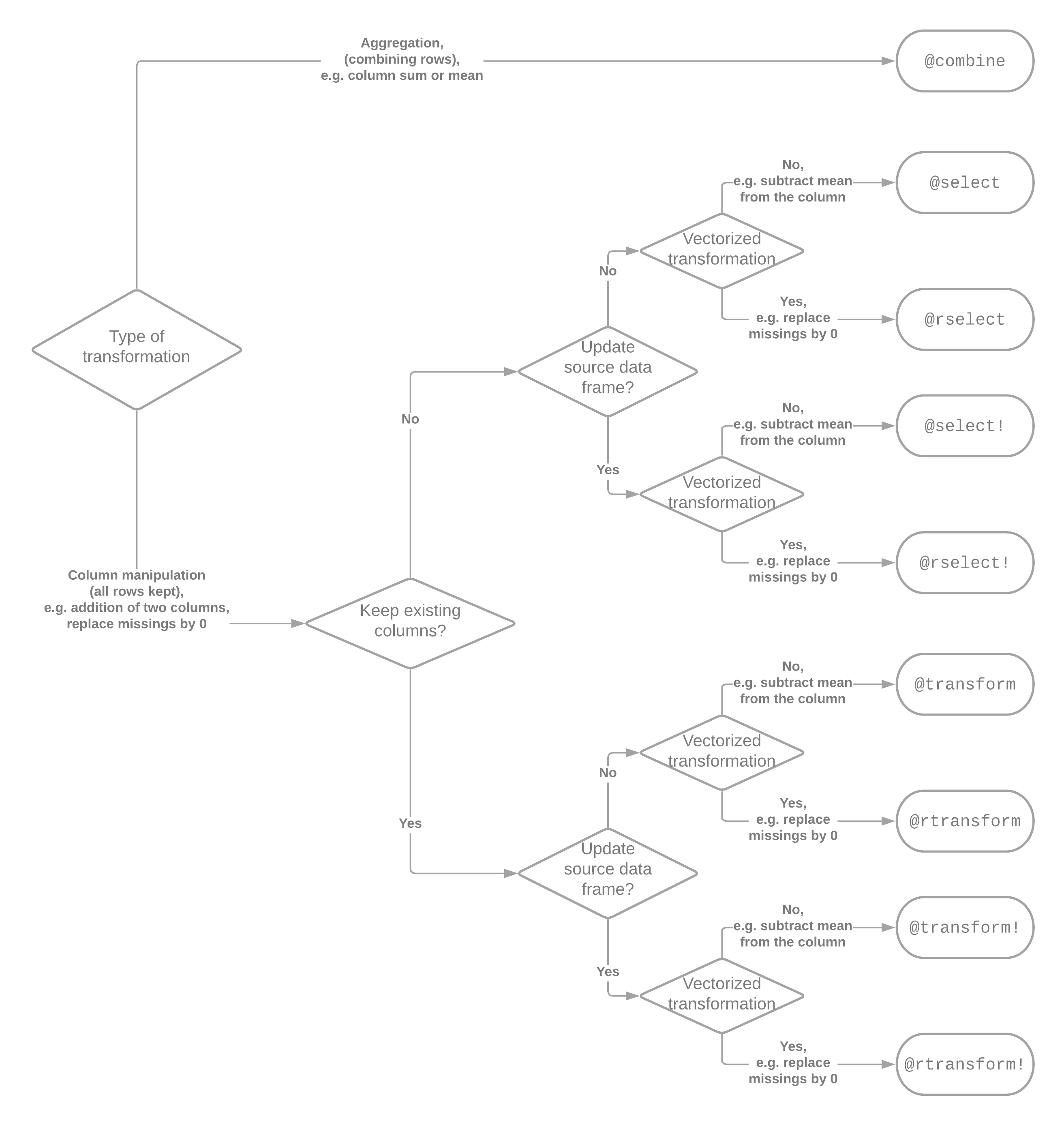
Today as a conclusion let me present the following flowchart summarizing the basic available data transformation options in DataFramesMeta.jl that I have covered:
There are many more features of DataFramesMeta.jl that I have not covered like: subsetting rows of a data frame, sorting it, or performing operations on grouped data. You can find all the details in the documentation of DataFramesMeta.jl.