Introduction

Last week Alan Edelman and Viral Shah had an excellent keynote talk during the Social Simulation Conference 2021. If you would like to learn about one of the models that was discussed about please read on.

My objective with this post is to make a permanent record of the model as, if I understood the comment of Alan Edelman correctly, it has not been published.

Of course all errors, extensions or omissions in the outline are mine (and I will gladly correct the post if they are any).

In the computational part of the post I use Julia 1.6.3, Roots.jl 1.3.5, and Plots.jl 1.22.3.

The problem statement

The question we want to answer is an attempt to address the the following empirical phenomenon:

Imagine there is a road accident. Assume it happened in a remote place where only one person is able to observe it. In such a situation it is highly likely that this person will try to help.

Now assume that the same accident happens in a densely populated area. Empirical data shows that each individual observer is much less likely to help, and even it is possible that the probability of any help drops in comparison to the first scenario when there is only one observer.

The model

The model of this situation that Alan Edelman presented is the following. Assume that we have \(n\) spectators of the event. Next we take that the baseline (i.e. when there is only one spectator) probability of helping is \(r\). Finally we define the probability multiplier \(f(n)>0\), where we assume that if there are \(n\) spectators each of them independently decides to help with probability \(f(n)r\). The assumptions about \(f\) are that \(f(1)=1\) and that \(f\) is decreasing.

Under these assumptions we can observe that the probability that any help is given is \(1-(1-f(n)r)^n\). We want to analyze the properties of this number. Now we fully switch from the social scientist’s hat to mathematician’s hat, by assuming \(n\to+\infty\).

Knife-edge condition

When we analyze the asymptotic properties of this model it is useful to define \(g(n)=f(n)n\). Then the formula for our probability becomes \(1-(1-g(n)r/n)^n\).

We now can notice that if \(g(n)\to0\) then the probability that help is given tends to \(0\). On the other hand if \(g(n)\to+\infty\) then the probability tends to \(1\).

So as we can see we get a sharp asymptotic knife-edge condition for the model of not being uninteresting. We get that the asymptotic probability is in \(]0,1[\) (assuming \(g(n)\) has a limit) only if \(g(n)\) has a positive and finite limit. In other words, asymptotically the probability of reaction of a spectator has to be proportional to \(1/n\). Assume that the limit is \(g\), i.e. \(g(n)\to g\). Then the asymptotic probability is \(1-\exp(-gr)\). So we might ask for which \(g\) the probability of reacting does not change. This is a solution to the equation \(r = 1-\exp(-gr)\). We can solve it to get \(g=-\log(1-r)/r\).

Now we are ready to jump into Julia to do some plotting.

Computational support

Let us now try plotting the solution of the equation \(r = 1-\exp(-gr)\) in \(g\) being a function of \(r\).

Here is the code that produces the requested plot:

julia> using Roots

julia> using Plots

julia> plot(r -> find_zero(g -> 1 - exp(-r * g) - r, 1.0),
            xlim=[0.01,0.99], xlabel="r", ylabel="g", legend=nothing)

and we get the following relationship:

g(r) plot

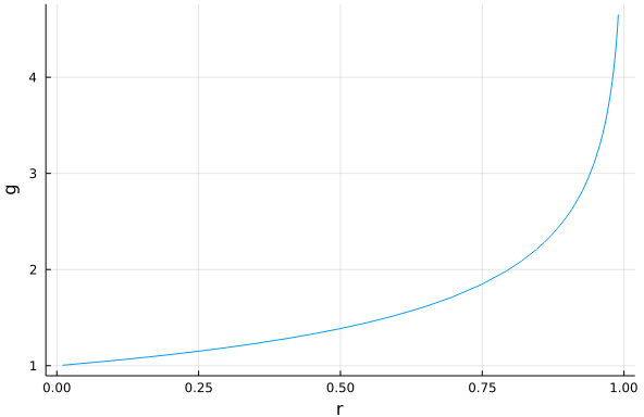
In the code above instead of using the analytical solution I have shown how one can dynamically find root of our equation as a function of a parameter.

As you can see the higher the initial \(r\) the higher \(g\) needs to be and it has to be greater than \(1\) in general.

Conclusions

I hope you enjoyed the post even though it was not that much about Julia. We have learned that the higher the baseline individual probability of reaction to some bad event the harder it becomes to keep the reaction probability at the given level as the number of spectators increases.