A tutorial on igraph for Julia

Introduction

I have been working with graphs both in Python and in Julia quite a lot recently. While I enjoy using LightGraphs.jl as it has a very lighweight and clean API its limitation is that it is missing some functionalities that are available in other packages like igraph.

In this post I want to comment on the basic steps for integrating both packages.

The examples are run under Linux, Julia 1.6, Cairo v1.0.5, Compose v0.9.2, GraphPlot v0.4.4, LightGraphs v1.3.5, and PyCall v1.92.2.

Before you start

You need to add igraph to your Python installation that is used by Julia using the following command:

using PyCall
run(`$(PyCall.python) -m pip install python-igraph`)

We will also use the partition_igraph package for community detection. It is installed using:

run(`$(PyCall.python) -m pip install partition_igraph`)

This package provides the ECG (ensemble clustering for graphs) algorithm that is a very nice approach to community detection. If you do not know it you might want to check out this and this papers.

The point of this post is that ECG is available only as a package for Python, so if you wanted to use it from Julia you need to use a bridge to igraph.

Getting the graph

We will want to use the standard Zachary’s karate club graph as an example. Let us start with loading the graph both in LightGraphs.jl and in igraph. First we load the required packages:

julia> using Cairo

julia> using Compose

julia> using GraphPlot

julia> using LightGraphs

julia> using PyCall

julia> using Random

julia> ig = pyimport("igraph");

julia> pyimport("partition_igraph");

Now load the graph both in LightGraphs.jl and in igraph:

julia> z_ig = ig.Graph.Famous("Zachary")
PyObject <igraph.Graph object at 0x7f5a18d49050>

julia> z_lg = smallgraph(:karate)
{34, 78} undirected simple Int64 graph

Let us check what is the mapping between these two graphs. The numbering of vertices in LightGraphs.jl is 1-based, whilie in igraph is 0-based. Let us check if in this case the mapping from z_lg to z_ig is just x -> x-1.

julia> nv(z_lg) == z_ig.vcount()
true

julia> ne(z_lg) == z_ig.ecount()
true

julia> z_lg_es = sort!(Tuple.(edges(z_lg)));

julia> z_ig_es = sort!([(e.source + 1, e.target + 1) for e in z_ig.es()]);

julia> z_lg_es == z_ig_es
true

Indeed in this case we see that the graphs are identical, as they have the same number of vertices, and the same edges. Note that I needed to sort! the edges collected to tuples as the iterators that produce these edges had a different ordering in both packages.

Note that it is also easy to write graph converters between LightGraphs.jl and igraph. Here is an example:

julia> function ig2lg(ig_g)
           lg_g = SimpleGraph(ig_g.vcount())
           for e in ig_g.es()
               add_edge!(lg_g, e.source + 1, e.target + 1)
           end
           return lg_g
       end
ig2lg (generic function with 1 method)

julia> ig2lg(z_ig)
{34, 78} undirected simple Int64 graph

julia> ig2lg(z_ig) == z_lg
true

The crucial thing to remember here is that LightGraphs.jl supports only simple graphs, so this property of the graph would have to be checked in igraph before doing the conversion. (similar operations can also be performed for directed simple graphs.)

Doing community detection

Now we move to the main point of our task. We want to run ECG algorithm on z_ig and then plot the z_lg graph using gplot function coloring its vertices using the communities found using ECG.

As ECG is randomized we run it 1,000 times and pick the split that maximizes modularity:

julia> ps = [z_ig.community_ecg().membership for i in 1:1000]; # generate partitions

julia> unique!(ps); # reduce as we have many duplicates

julia> mps = z_ig.modularity.(ps); # calculate modularity for each partition

julia> bestp = ps[argmax(mps)] .+ 1; # get the best partition

Note how easy it is to mix Python functionality with Julia in the above code. In the last line I add 1 to the resulting vector to make in 1-based.

Finally we save the plot of the graph to a PNG file:

julia> cls = ["red","green","blue", "pink", "black"]; # we allow up to 5 communities

julia> Random.seed!(12);

julia> z_plot = gplot(z_lg,
                      NODESIZE=0.03, nodefillc=cls[bestp],
                      EDGELINEWIDTH=0.2, edgestrokec="gray");

julia> draw(PNG("z_plot.png"), z_plot);

Note that the mapping between z_ig and z_lg is just x -> x + 1 we do not have to reorder the bestp vector.

This is the plot you should get:

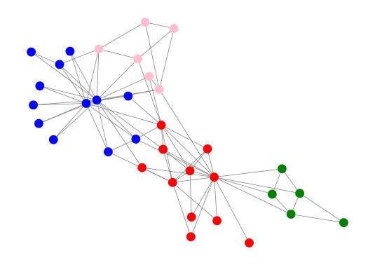
As you can see the ECG algorithm seems to have identified the communities in the graph reasonably well.

Conclusions

As you can see integration between LightGraphs.jl and igraph is very easy. The major things you have to keep in mind when using it are:

• igraph uses 0-based intexing, while LightGraphs.jl is 1-based;
• always make sure what transformation of vertex indices you should use to map vertex numbers between igraph and LightGraphs.jl (a natural one is just x -> x + 1 if they are stored in the same order);
• edges might be stored in both packages in a different order;
• make sure to check if you are working with a graph or a digraph and use a proper graph type in LightGraphs.jl;
• remember that LightGraphs.jl only supports simple graphs.

I hope this post will help you to get started with igraph integration if you might need to use it!