Introduction

After my last post on random number generation I think that it is good to add one more thing that Chris Rackauckas pointed out to me as relevant to show a complete picture. If you are working with pseudo random number generators it is good to know that Julia has an excellent RandomNumbers.jl package that offers a wide array of different random number generators to choose from. So in this post I will use xoroshiro128** generator.

The post was tested under Julia 1.5.3 and packages DataFrames.jl 0.22.1, Distributions.jl 0.23.8, FreqTables.jl 0.4.2, Pipe.jl 1.3.0, RandomNumbers.jl 1.4.0, PyPlot.jl 2.9.9 and intends to present a pretty complete work-flow of investigating a sample data science problem.

A/B testing

In the post we will investigate several simple options how A/B tests can be performed.

In our scenario we assume that we have to choose from \(n\) alternatives. Each alternative \(i\in[n]\) has an unknown probability of success \(p_i\). Assume that e.g. we have \(n\) different ways to promote a product to a customer and \(p_i\) is a probability that customer buys after seeing a promotion.

Initially we do not know which of the options is the best, i.e. has the highest \(p_i\), but we are allowed to present them to customers and collect their responses to learn the unknown probabilities.

The most simple way to run such an experiment is to present each option to the customer with the same probability \(1/n\). Such an approach focuses purely on exploration of the alternatives. However, intuitively we feel that it is wasteful. If after some trials we see that some option is very bad and has marginal chances of being the best then it is not worth showing it to the customer. We are not only losing money (we present something that we know is not very good), but additionally we will not learn much in terms of choosing the best option.

Another approach would be to always show our customer an option that we currently believe is best. Such a strategy focuses purely on exploitation. Similarly to the uniform sampling described above, we can see that it does not have to lead to good outcomes. We can get stuck with sub-optimal solution, as we do not give ourselves a chance to learn that maybe some alternative that is currently not considered the best is actually superior.

So how can we balance the exploration with exploitation? There are many approaches that can be considered, but one of the simplest, yet very efficient, is Thompson sampling. In this approach we do the following. We constantly keep information about the distribution of our beliefs about the quality of each alternative. Denote the random variable corresponding to the distribution of these beliefs as \(P_i\) for alternative \(i\). Now in each step we independently sample a value from each distribution \(P_i\) and choose to measure the option that has the highest value of the sample. Now why does this heuristic work? Note that we will tend to sample the alternatives that have a high value of beliefs (so we do not waste time on sampling very bad options) but at the same time we will also from time to time sample options that have a high variance of \(P_i\) distribution (so the options about which we do not know much; even if at the moment of sampling we believe they are not so good our beliefs show us that actually they could turn out good if we collect more evidence on them).

In the codes below I compare these three strategies of running A/B tests. I call them respectively:

Uniform: sample each alternative with probability \(1/n\);
Greedy: sample the alternative with the highest \(E(P_i)\);
Thompson: sample the alternative with the highest value of a single independent sample from \(P_i\).

Before we turn to coding one last thing should be discussed. How should we represent our beliefs \(P_i\)? Fortunately here Bayesian statistics comes handy. As our experiments are Bernoulli trials, we know that if we represent the prior beliefs as Beta distributed then the posterior beliefs are also going to follow the same distribution. Formally we say that the Beta distribution is a conjugate prior of Bernoulli distribution. If our beliefs have \(Beta(\alpha, \beta)\) distribution and we see a success then the distribution of beliefs becomes \(Beta(\alpha+1, \beta)\). On the other hand if we see a failure it becomes \(Beta(\alpha, \beta+1)\). As you can see it is very easy to implement.

Setting up the stage

In a fresh Julia session we first load the required packages:

using DataFrames
using Distributions
using FreqTables
using Pipe
using RandomNumbers
using PyPlot
using LinearAlgebra

Next define a function that updates the beliefs about the quality of some alternative:

update_belief(b::Beta, r::Bool) = Beta(b.α + r, b.β + !r)

Finally define the three decision rules that we want to compare: uniform, greedy, and Thompson:

abstract type ABRule end

struct Greedy <: ABRule end
struct Thompson <: ABRule end
struct Unif <: ABRule end

function decide(options::Vector{<:Beta}, ::Unif)
    return rand(axes(options, 1))
end

function decide(options::Vector{<:Beta}, ::Greedy)
    m = mean.(options)
    mm = maximum(m)
    return rand(findall(==(mm), m))
end

function decide(options::Vector{<:Beta}, ::Thompson)
    m = rand.(options)
    mm = maximum(m)
    return rand(findall(==(mm), m))
end

One technical aspect of our implementations of decision making rule for greedy and Thompson sampling is that we have to take into consideration that more than one option can have the same evaluation. That is why we need first to find which option has maximum mean with mm = maximum(m) and then randomly select one of the options that are best with rand(findall(==(mm), m)).

Now we are ready to run the experiment.

Implementing the experimenter

Here is an implementation of the function that runs the experiments:

function coupled_run!(n::Int, steps::Int, rng::AbstractRNG,
                      results::DataFrame, runid::Int)
    truep = rand(rng, n)
    bestp = argmax(truep)
    streams = [rand(rng, Bernoulli(p), steps) for p in truep]

    for alg in (Greedy(), Unif(), Thompson())
        options = [Beta(1, 1) for i in 1:n]
        loc = fill(1, n)
        for i in 1:steps
            d = decide(options, alg)
            options[d] = update_belief(options[d], streams[d][loc[d]])
            loc[d] += 1
        end
        push!(results, (runid=runid, alg=string(typeof(alg)),
                        correct=mean(options[bestp]) == maximum(mean.(options)),
                        payoff=sum(x -> x.α - 1, options)))
    end
end

The coupler_run! takes five arguments: k is number of alternatives to consider, steps is the length of A/B test experiment, rng is random number generator we will use (remember that we want to test RandomNumbers.jl library), results is a data frame that we will update and store the experiment results in, finally runid is experiment number.

Let us comment on several crucial parts of the above code. Note that we sample unknown true probabilities of success in the experiment with truep = rand(rng, n). As they are uniformly distributed we set our initial beliefs about options to also follow a uniform distribution in this line: options = [Beta(1, 1) for i in 1:n].

The next notable thing is that we want the experiments for all algorithms we consider to be coupled, that is: each alternative should generate the same sequence of successes and failures for each option. Therefore, for simplicity, we pre-populate the results of the trials in this line streams = [rand(rng, Bernoulli(p), steps) for p in truep] and then just tack in loc vector which random number for each option should be picked. Such an approach will reduce noise when comparing the alternatives. (note that we could have implemented it more efficiently, but I did not want to over-complicate the code).

Finally note that we are collecting two informations:

correct: if what we think is best at the end of the experiment is best indeed.
payoff: how much payoff we have collected when running the experiment.

Note that both of them are desirable. Everyone probably agrees that it would be best to have correct near to one (so that after running the experiment we are confident that we know what is best). At the same time it is also desirable to ensure that the experiment itself is not wasteful, so that we collect as big payoff as possible.

We will compare the three considered A/B testing rules using these two criteria.

Analyzing the experiment results

First run the experiment (it should take under 20 seconds):

julia> results = DataFrame()
0×0 DataFrame

julia> rng = Xorshifts.Xoroshiro128StarStar(1234)
RandomNumbers.Xorshifts.Xoroshiro128StarStar(0x9e929e92000004d2, 0xda409a400013489a)

julia> @time foreach(runid -> coupled_run!(10, 500, rng, results, runid), 1:20_000)
 18.736959 seconds (143.71 M allocations: 8.944 GiB, 6.78% gc time)

julia> results
60000×4 DataFrame
   Row │ runid  alg       correct  payoff
       │ Int64  String    Bool     Float64
───────┼───────────────────────────────────
     1 │     1  Greedy      false    451.0
     2 │     1  Unif         true    354.0
     3 │     1  Thompson     true    486.0
     4 │     2  Greedy       true    468.0
     5 │     2  Unif         true    264.0
   ⋮   │   ⋮       ⋮         ⋮        ⋮
 59997 │ 19999  Thompson     true    464.0
 59998 │ 20000  Greedy      false    472.0
 59999 │ 20000  Unif         true    394.0
 60000 │ 20000  Thompson     true    462.0
                         59991 rows omitted

We have run the sampling 20,000 times in under 20 seconds. We have 60,000 rows in our DataFrame as for each sampling we produced three rows corresponding to three alternatives we consider. In our experiment we considered 10 alternatives and a budget of 500 samples for testing.

First we collect some initial statistics about the alternatives:

julia> @pipe groupby(results, :alg) |>
             combine(_, [:correct, :payoff] .=> mean)
3×3 DataFrame
 Row │ alg       correct_mean  payoff_mean
     │ String    Float64       Float64
─────┼─────────────────────────────────────
   1 │ Greedy         0.38145      405.997
   2 │ Unif           0.8031       250.394
   3 │ Thompson       0.87955      431.31

We see that Thompson sampling has both best probability of being correct and the best cumulative payoff. Interestingly greedy strategy has low probability of being correct, but relatively high payoff. The opposite holds for uniform sampling strategy.

Now we investigate correct selection probability in more detail:

julia> correct_wide = unstack(results, :runid, :alg, :correct)
20000×4 DataFrame
   Row │ runid  Greedy  Unif   Thompson
       │ Int64  Bool?   Bool?  Bool?
───────┼────────────────────────────────
     1 │     1   false   true      true
     2 │     2    true   true      true
     3 │     3   false   true      true
     4 │     4   false   true      true
     5 │     5   false  false     false
   ⋮   │   ⋮      ⋮       ⋮       ⋮
 19997 │ 19997   false   true      true
 19998 │ 19998   false  false      true
 19999 │ 19999   false   true      true
 20000 │ 20000   false   true      true
                      19991 rows omitted

julia> proptable(correct_wide, :Greedy, :Unif)
2×2 Named Array{Float64,2}
Greedy ╲ Unif │   false     true
──────────────┼─────────────────
false         │ 0.14145   0.4771
true          │ 0.05545    0.326

julia> proptable(correct_wide, :Greedy, :Thompson)
2×2 Named Array{Float64,2}
Greedy ╲ Thompson │   false     true
──────────────────┼─────────────────
false             │  0.0907  0.52785
true              │ 0.02975   0.3517

julia> proptable(correct_wide, :Unif, :Thompson)
2×2 Named Array{Float64,2}
Unif ╲ Thompson │   false     true
────────────────┼─────────────────
false           │  0.0893   0.1076
true            │ 0.03115  0.77195

Observe that Thompson and uniform sampling give quite similar results most of the time , with Thompson sampling having a slight edge when they disagree. Greedy strategy is much worse. It is easy to understand these findings. Greedy strategy is not doing enough exploration. Both Thompson and uniform sampling do explore. The edge of Thompson sampling is that it does not waste time testing very bad alternatives (so it can focus on the good ones and better discriminate between them).

Similarly we can investigate which alternative gives the best payoff (remember that we made sure to have the scenarios coupled):

julia> function find_best(alg, payoff)
           best_idxs = findall(==(maximum(payoff)), payoff)
           best_algs = alg[best_idxs]
           sort!(best_algs)
           return join(best_algs, '|')
       end
find_best (generic function with 1 method)

julia> alg_freq = @pipe groupby(results, :runid) |>
                        combine(_, [:alg, :payoff] => find_best => :best) |>
                        groupby(_, :best, sort=true) |>
                        combine(_, nrow)
3×2 DataFrame
 Row │ best             nrow
     │ String           Int64
─────┼────────────────────────
   1 │ Greedy            9736
   2 │ Greedy|Thompson    120
   3 │ Thompson         10144

We observe that uniform sampling for 20,000 simulations was never the best, while Thompson sampling has a slight edge over greedy sampling in the probability of being best (there is also a small probability of a tie).

As an exercise let us check, sticking to Bayesian approach, what is the probability that Thompson sampling has higher probability of being best than greedy one. Here we use the fact that the Dirichlet distribution is a conjugate prior for the Categorical distribution, and set uniform a priori beliefs:

julia> posterior = Dirichlet(alg_freq.nrow .+ 1)
Dirichlet{Float64}(alpha=[9737.0, 121.0, 10145.0])

julia> posterior_dis = rand(rng, posterior, 100_000)
3×100000 Array{Float64,2}:
 0.484744    0.486453    0.492359    …  0.494059   0.484432    0.482332
 0.00632059  0.00692795  0.00563844     0.0076129  0.00706873  0.00782947
 0.508936    0.506619    0.502002       0.498328   0.508499    0.509838

julia> mean(x -> x[1] < x[3], eachcol(posterior_dis))
0.99707

We can see that given the sample size of 20,000 this probability is greater than 99%.

However, we see that the considered fractions actually do not differ that much:

julia> transform(alg_freq, :nrow => (x -> x ./ sum(x)) => :freq)
3×3 DataFrame
 Row │ best             nrow   freq
     │ String           Int64  Float64
─────┼─────────────────────────────────
   1 │ Greedy            9736   0.4868
   2 │ Greedy|Thompson    120   0.006
   3 │ Thompson         10144   0.5072

and the difference in average payoffs we observed above was relatively higher. Let us dig into this. First we plot a distribution of difference between payoffs with Thompson and greedy sampling:

payoff_wide = unstack(results, :runid, :alg, :payoff)
Δpayoff = payoff_wide.Thompson .- payoff_wide.Greedy
hist(Δpayoff, 25)
xlabel("Δpayoff: Thompson-Greedy")

getting the following plot:

Delta of payoff

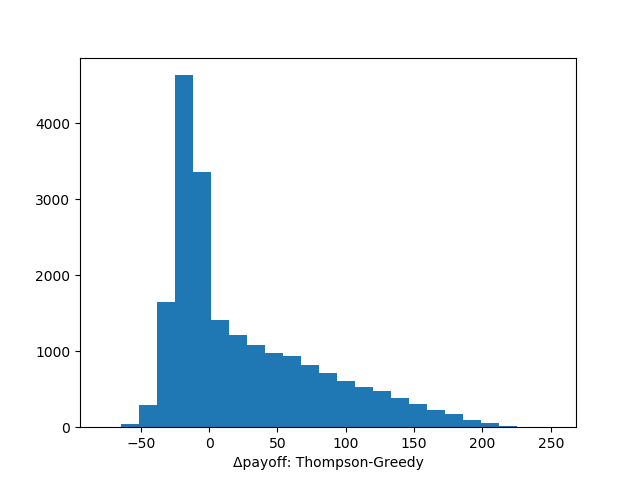
Now we see what is going on. If Thompson sampling is worse than greedy sampling it is worse only slightly. On the other hand greedy sampling can be much worse than Thompson sampling (and we understand when: this is a scenario when greedy algorithm gets stuck at some sub-optimal alternative).

We also quickly check the distribution of estimator of the difference in payoffs using Bayesian bootstrapping (to keep to the style we use in this post):

julia> dd = Dirichlet(length(Δpayoff), 1);
julia> boot = [dot(Δpayoff, rand(rng, dd)) for _ in 1:10_000];

julia> quantile(boot, 0:0.25:1)
5-element Array{Float64,1}:
 23.427965439713827
 24.64825057737705
 24.911299035010433
 25.17170629935465
 26.513561155964837

and we see, that, as expected the distribution of the difference is very significantly greater than zero (we could probably easily detect this significance even with a much smaller number of tests than 20,000).

Conclusion

That was a long post, so let me finish at this point. I hope you enjoyed it and could also appreciate the data wrangling capabilities that JuliaData ecosystem offers you. I also encourage you to run some more experiments on your own to chcek how the considered A/B testing strategies behave under different parameterizations.

And a usual caveat – performance geeks (are there any in the Julia community?) can find several spots in my codes that I left sub-optimal to keep them simple. Feel free to experiment with improving the execution speed of my examples.