Writing an AR(1) process simulator as a module in Julia

ABC of modules in Julia

Modules in Julia allow you to create separate variable workspaces. You can find all the details needed to work with modules in the Julia Manual.

In this post let me focus on one of the reasons to create modules in your programs: you can control which names defined in the module get exposed outside the module.

In order to show this let us create a simple AR(1) process simulator, to see some story — not just dry definitions. For completeness we will first introduce a bit of theory of such processes, next we will discuss how you can define your own module, and finally we will show how we can use it.

This post was prepared under Julia 1.4.2 and is mostly targeted at people who want to start using Julia for doing computation-heavy operations (therefore I allow myself to drift away and comment on many things that are are not a core of the example we give, but are a natural questions that arise in practice when writing similar codes).

AR(1) model definition

The AR(1) model is a random process \(X_t\), where \(t\in\mathbb{Z}\), and the support of random variables \(X_t\) is \(\mathbb{R}\), that follows the equation:

\[X_t = c + \phi X_{t-1} + \varepsilon_t,\]

where \(\varepsilon_i\) are independent random variables that are normally distributed with mean \(0\) and variance \(\sigma^2\).

For the AR(1) process to be stationary we assume \(|\phi|<1\). Also clearly we have \(\sigma\geq0\), as standard deviation must be non-negative.

We will want to create a simulator of this process in Julia.

In order to implement it we need to derive the distribution of the unconditional mean and variance of \(X_t\). It is simplest to get them assuming they exist and are independent from \(t\) (they do as we take \(|\phi|<1\); I omit some technical details here).

For expected value we get:

\[E(X_t) = E(c + \phi X_{t-1} + \varepsilon_t) = c + \phi E(X_{t-1}).\]

but as the process is stationary \(E(X_t)=E(X_{t-1})\) so after substituting \(E(X_t) = c / (1 - \phi)\).

For variance we get:

\[D^2(X_t) = D^2(c + \phi X_{t-1} + \varepsilon_t) = \phi^2 D^2(X_{t-1}) + \sigma^2,\]

where we have used the assumption that \(\varepsilon_t\) is independent from \(X_{t-1}\). Again, as the process is stationary \(D^2(X_t)=D^2(X_{t-1})\) so after substituting \(D(X_t) = \sigma^2 / (1 - \phi^2)\).

The last question is what is the unconditional distribution of \(X_t\). We know its mean and variance (and they are both finite), so it is easiest to unroll the AR(1) process definition recursively \(s\) times:

\[X_t = c + \phi X_{t-1} + \varepsilon_t = \ldots = \phi^{s+1}X_{t-s+1} + \sum_{i=0}^s \phi^i (c + \varepsilon_{t-i})\]

Since we know that \(X_{t-s+1}\) has a finite variance we see that if we let \(s\to\infty\) then \(X_t\) converges in probability to a normal distribution (here we use the fact that \(\varepsilon_i\) are normally distributed and a sum of normally distributed variables is also normally distributed). In conclusion we get that:

\[X_t \sim \mathcal{N}\left(\frac{c}{1-\phi},\frac{\sigma^2}{1-\phi^2}\right).\]

Definiing a module with a AR(1) simulator

First let me show a complete way how I would normally define such a simulator. Below I discuss some of practices that are present in the code.

module AR1

using Random

export ar1!, ar1

const AR1_COMMON_DOC = """
elements following the AR(1)
process where `xₜ₊₁ = c + ϕxₜ + εₜ` and `εₜ ∼ N(0, σ²)`.

If `start` keyword argument is passed then this is the first element of the
returned vector. Otherwise it is initiated randomly to follow the stationary
distribution of the process.


You can pass `rng` keyword argument to specify a custom random number generator
that should be used when generating data.

It is required that |ϕ| < 1 so that the process is stationary.
"""

sample_start(c::Real, ϕ::Real, σ::Real, rng::AbstractRNG) =
    c / (1 - ϕ) + randn(rng) * σ / sqrt(1 - ϕ^2)

"""
    ar1!(v, c, ϕ, σ; rng, start)

Update vector `v` in place by filling it with
$AR1_COMMON_DOC
"""
function ar1!(v::AbstractVector{<:AbstractFloat}, c::Real, ϕ::Real, σ::Real;
              rng::AbstractRNG=Random.default_rng(),
              start::Real=sample_start(c, ϕ, σ, rng))
    σ < 0 && throw(ArgumentError("σ is not allowed to be negative"))
    abs(ϕ) < 1 || throw(ArgumentError("|ϕ| < 1 is required"))
    x = start
    n = length(v)
    if n > 0
        v[1] = x
        for i in 2:n
            x = c + x * ϕ + randn(rng) * σ
            v[i] = x
        end
    end
    return v
end

"""
    ar1(n, c, ϕ, σ; rng, start)

Return a vector containing `n`
$AR1_COMMON_DOC
"""
function ar1(n::Integer, c::Real, ϕ::Real, σ::Real;
             rng::AbstractRNG=Random.default_rng(),
             start::Real=sample_start(c, ϕ, σ, rng))
    return ar1!(Vector{Float64}(undef, n), c, ϕ, σ, rng=rng, start=start)
end

end # module

First let us start with a discussion why we want to use a module for this code at all. The reason is that inside the module we define a constant AR1_COMMON_DOC and three functions: sample_start, ar1! and ar1. However, I do not want AR1_COMMON_DOC nor sample_start to be exposed to users. They are just an internal implementation detail, therefore only ar1! and ar1 are exported from the module.

Also the module loads a standard module Random. Though unlikely, some codes that will want to use my AR1 module might not to have Random module loaded. Since using Random is wrapped inside the module I can use Random inside the AR1 module but it is not visible outside the module (unless you explicitly import it of course).

Now let me comment on some other things that are present in this code (and maybe you will find these practices useful):

• I define AR1_COMMON_DOC as a constant string that gets interpolated into docstings of ar1! and ar1. This is the part of the documentation that is common for the two methods. I have found that if you need to maintain some code in the long term it is really useful to do this. Otherwise, especially if your code base is large, it is really easy to have a situation that the documentation gets out of sync.
• I define the sample_start function as it is called both in ar1! and ar1 to set the default value of start parameter. Again, having it extruded makes it simpler to maintain the code in the long term (you need to change the code only in one place).
• In ar1! and ar1 I allow the users to pass their own PRNG, which is often needed when one wants to use some more advanced techniques of stochastic simulation (like e.g. variance reduction). However, I still want the user not to have to pass it by default, but use the generator that is provided by default by the Random module. Note that by using Random.default_rng() on Julia 1.4.2 I am sure that my code is thread safe.
• I implement ar! function that works in-place and an ar1 function that allocates a fresh output vector on each call. This is a common pattern in Julia and we will investigate its performance consequences later in this post.
• Note that in all functions I give the constraints on the allowed types and values of their parameters. However, in ar1 I create the initial vector as Vector{Float64}(undef, n) (i.e. it has Float64 elements) because randn in Julia produces Float64 output by default. Still in ar1! I allow v to be AbstractVector{<:AbstractFloat} as in some applications the user might want to pass a vector of other type (e.g. located in GPU memory and containing Float32 elements; note though that in such a scenario probably one could consider replacing randn(rng) calls by its more efficient version for performance reasons).
• In operations in hot loops like v[i] = x in the ar1! function I often see people use @inbounds. I personally try to avoid this. The performance gain is usually not that big, and it is very common that one thinks that using @inbounds is safe, while in practice there is some bug in the code and it is not (you can always pass --check-bounds=no switch when starting your Julia session to disable bounds checking later).
• I opted to make rng and start keyword arguments. The reason is that most likely the user will want to omit specifying them. Note that the rng is defined before start keyword argument, because we use rng to calculate the default value of start if it would not be provided by the user.
• I always use return explicitly in functions defined with function keyword argument as in the long term it is more readable.
• Finally, at least for me, it is very nice that it is really easy to use variable names like ϕ or σ in the code (and also type them in the editor or REPL). Not only it makes functions match my math formulas, but also the lines are shorter.

Uff, the list was longer than the code :).

Before we start

Before we start make sure that you have the packages that we will installed in the right versions. We will use: StatsBase.jl v0.32.2 and PyPlot.jl v2.9.0.

First start your Julia REPL with the command, in Linux:

$ JULIA_NUM_THREADS=2 julia

and in Windows

C:\> set JULIA_NUM_THREADS=2
C:\> julia

(what we do here is informing Julia that it can use two threads for computations — we will soon use it; I have chosen two threads as I assume most current computers have at least two cores so that everyone should be able to follow this setting)

You can check if you have the packages in the right versions by switching to package manager mode in the Julia REPL (press ] to do it) and writing: status command. If you do not have them or the versions are incorrect while still in the package manager mode write the following commands (I assume that you do not have Project.toml and Manifest.toml files in your current working directory):

(@v1.4) pkg> activate .
 Activating new environment at `~/Project.toml`

(bkamins) pkg> add StatsBase@0.32.2
...

(bkamins) pkg> add PyPlot@2.9.0
...

(bkamins) pkg> status
Status `~/Project.toml`
  [d330b81b] PyPlot v2.9.0
  [2913bbd2] StatsBase v0.32.2

(I have removed the output that some commands produce as it is not required for our purposes).

Now we are all set to test our code. Exit the package manager mode by pressing a backspace.

Using AR(1) simulator

First copy paste the code containing the AR1 module definition to your Julia REPL.

In order to use the module write:

julia> using .AR1

Note that it is crucial to write a . before the module name as the module is defined in the current global scope of so called Main module (you should have seen Main.AR1 printed when you pasted the definition of the module in the Julia REPL).

You were probably using statements like using Random (like we did in the code of the AR1 module). This way of loading modules searches for them in standard library or installed packages. In our case we have a custom module defined only in this session, so we need to add . to allow Julia to locate it.

After making the using statement we can use ar1 and ar1! functions. Let us first check the help for ar1 (to make sure it correctly incorporates the AR1_COMMON_DOC string). Press ? in the Julia REPL, write ar1 and press enter to get:

help?> ar1
search: ar1 ar1! AR1 @macroexpand1

  ar1(n, c, ϕ, σ; rng, start)

  Return a vector containing n elements following the AR(1) process where
  xₜ₊₁ = c + ϕxₜ + εₜ and εₜ ∼ N(0, σ²).

  If start keyword argument is passed then this is the first element of the
  returned vector. Otherwise it is initiated randomly to follow the
  stationary distribution of the process.

  You can pass rng keyword argument to specify a custom random number
  generator that should be used when generating data.

  It is required that |ϕ| < 1 so that the process is stationary.

We conclude that all looks as expected.

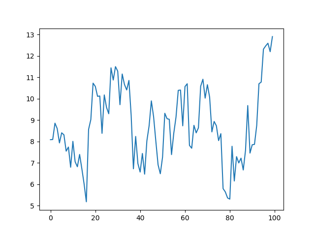
As a fist task let us plot one sample of our simulator output:

julia> using PyPlot

julia> plot(ar1(100, 1, 0.9, 1))

You should get a plot similar to (it will not be identical, as we did not set the seed of the random number generator; in all the results that follow you should expect the same situation — they should be similar but probably not identical to what I show):

Next let us check if indeed \(\phi=0.9\) for the process we considered. For this let us generate a longer data set to have the results more accurate:

julia> using StatsBase

julia> autocor(ar1(10^6, 1, 0.9, 1), 1:1)
1-element Array{Float64,1}:
 0.9003360673839191

and we get a value very close to 0.9 as expected.

Now let us discuss why we have cared so much about deriving the formula for the stationary distribution of \(X_t\). Note that we use this formula to set the default value of start variable. The consequence should be that if we generate a random AR(1) vector many times all its elements should have a mean of around \(1/(1-0.9)=10\) and variance of around \(1/(1-0.9^2)=100/19\approx 5.26316\).

Let us check it for a default start:

using Statistics

julia> sim = [ar1(100, 1, 0.9, 1) for i in 1:10^6];

julia> extrema(mean.([getindex.(sim, i) for i in 1:100]))
(9.996782972052698, 10.003866043483425)

julia> extrema(var.([getindex.(sim, i) for i in 1:100]))
(5.2518154979875575, 5.2742608590894475)

and indeed we see that the results are correct.

If we would set start to be equal to the expected mean, but non-random, then we will get a visible bias in the variance of the first few observations (but the mean will be correct):

julia> sim = [ar1(100, 1, 0.9, 1, start=10) for i in 1:10^6];

julia> extrema(mean.([getindex.(sim, i) for i in 1:100]))
(9.996503785236944, 10.00565659110953)

julia> extrema(var.([getindex.(sim, i) for i in 1:100]))
(0.0, 5.2751198890482005)

julia> plot(var.([getindex.(sim, i) for i in 1:100]))

and the generated plot of variance looks like this:

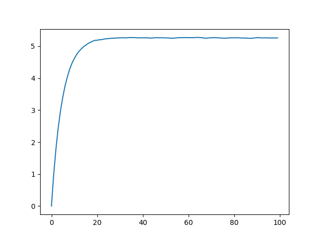
Setting start to be biased will similarly bias the first few expectations in the generated process.

Performance considerations

As a performance test assume that we were interested in running the mean test but not for \(10^6\) but \(10^8\) repetitions to get more accurate results. The problem is that in that case we would need memory roughly of order \(8\cdot 100 \cdot 10^8\) bytes, which is 80GiB (not something I can store in RAM of my laptop).

A basic code that does such a check, while not having to store all the generated data, could look like this:

function f1(n::Integer)
    s = zeros(100)
    for i in 1:n
        s .+= ar1(100, 1, 0.9, 1)
    end
    return extrema(s) ./ n
end

Let us test it (the first run is supposed to compile the function to give more accurate results for the second run):

julia> @time f1(100)
  0.000087 seconds (101 allocations: 88.375 KiB)
(9.508060461092601, 10.437892560883078)

julia> @time f1(10^8)
107.395185 seconds (100.00 M allocations: 83.447 GiB, 10.97% gc time)
(9.99928784783692, 10.000313949053089)

So we we need around 100 seconds to finish, and indeed a bit over 80GiB of data got allocated. Can we do better?

In the first step let us try to avoid some allocations by using ar1! instead of ar1:

function f2(n::Integer)
    s = zeros(100)
    v = zeros(100)
    for i in 1:n
        s .+= ar1!(v, 1, 0.9, 1)
    end
    return extrema(s) ./ n
end

and test shows the following:

julia> @time f2(100)
  0.000081 seconds (2 allocations: 1.750 KiB)
(9.54394702371765, 10.480846071057933)

julia> @time f2(10^8)
 62.640395 seconds (2 allocations: 1.750 KiB)
(9.999306112039276, 10.000679734746692)

Indeed — we have almost halved the run time.

Let us finally turn to threading (the JULIA_NUM_THREADS=2 option that was quietly waiting for being used from the beginning of our session):

function f3(n::Integer)
    s = [zeros(100) for _ in 1:Threads.nthreads()]
    v = [zeros(100) for _ in 1:Threads.nthreads()]
    Threads.@threads for i in 1:n
        tid = Threads.threadid()
        s[tid] .+= ar1!(v[tid], 1, 0.9, 1)
    end
    return extrema(sum(s)) ./ n
end

Let us check if all went as we expected:

julia> Threads.nthreads()
2

julia> @time f3(100)
  0.000137 seconds (21 allocations: 6.078 KiB)
(9.452653560199144, 10.31887937207082)

julia> @time f3(10^8)
 36.220213 seconds (21 allocations: 6.078 KiB)
(9.999318657341107, 10.000619565457022)

Using 2 threads we have almost halved the computation time. Note that this time we have allocated separate vectors for each thread and accessed them using the tid variable to avoid race condition issues.

Most common problem when using modules

Before we finish let us comment on a thing that people often find confusing then working with modules. Here we will just use the modules that are present by default in a standard Julia REPL session: Main (where all your work happens) and Base (containing the definitions of standard functions you can normally use without importing anything). In particular functions sin and cos are defined in Base module. Now consider the following example:

julia> sin(1)
0.8414709848078965

julia> sin = 2
ERROR: cannot assign a value to variable Base.sin from module Main
Stacktrace:
 [1] top-level scope at REPL[5]:1

julia> cos = 2
2

julia> cos(1)
ERROR: MethodError: objects of type Int64 are not callable
Stacktrace:
 [1] top-level scope at REPL[7]:1

julia> Base.cos(1)
0.5403023058681398

In the case of sin you first call sin(1) which makes Julia associate name sin in module Main with the function sin defined in module Base. So later when trying to set a value of 2 to sin you get an error (name sin is now bound to a function and you are not allowed to change its meaning).

For the other case for cos you give it a value in module Main first. From that moment cos is bound to 2 (of course you could change this binding later), which overshadows the function with name cos from module Base. As you can see in such a case to call cos from Base you have to qualify its name and write Base.cos(1).

In short — when importing names from other modules be careful about using duplicate names (it is best just not to use the names you decided to import from other modules).

---

 

If you are still with me — thank you for reading the post and I hope you enjoyed it!